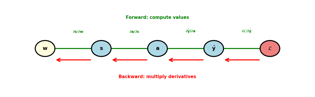
Training Neural Networks Requires Gradients
Single variable: \(y = f(g(x))\):
\[\frac{dy}{dx} = \frac{df}{dg} \cdot \frac{dg}{dx}\]
“Deep” composition: \(y = f(g(h(x)))\):
\[\frac{dy}{dx} = \frac{df}{dg} \cdot \frac{dg}{dh} \cdot \frac{dh}{dx}\]
Backpropagation applies chain rule systematically: Each layer computes local derivative. Composition handled by passing gradients backward.
Deep network with \(L\) layers: \(\frac{\partial \mathcal{L}}{\partial \mathbf{w}^{(1)}}\) requires \(L\) chain rule applications. Direct computation: 1 forward pass + 1 backward pass.
Composition in Deep Networks
Two-layer network:
\[\mathbf{x} \xrightarrow{W^{(1)}} \mathbf{s}^{(1)} \xrightarrow{\sigma} \mathbf{a}^{(1)} \xrightarrow{W^{(2)}} \mathbf{s}^{(2)} \xrightarrow{\sigma} \hat{y}\]
Forward pass equations:
Layer 1:
\[\mathbf{s}^{(1)} = W^{(1)}\mathbf{x} + \mathbf{b}^{(1)}\]
\[\mathbf{a}^{(1)} = \sigma(\mathbf{s}^{(1)})\]
Layer 2:
\[\mathbf{s}^{(2)} = W^{(2)}\mathbf{a}^{(1)} + \mathbf{b}^{(2)}\]
\[\hat{y} = \sigma(\mathbf{s}^{(2)})\]
Loss:
\[\mathcal{L} = -[y\log \hat{y} + (1-y)\log(1-\hat{y})]\]
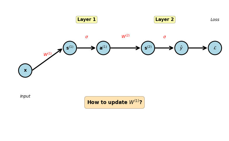
Question: How to update \(W^{(1)}\)?
Answer: \(W^{(1)} \leftarrow W^{(1)} - \eta \frac{\partial \mathcal{L}}{\partial W^{(1)}}\)
Loss depends on \(W^{(1)}\) through path:
\[\mathcal{L} \leftarrow \hat{y} \leftarrow \mathbf{s}^{(2)} \leftarrow \mathbf{a}^{(1)} \leftarrow \mathbf{s}^{(1)} \leftarrow W^{(1)}\]
Need systematic method for arbitrary depth
Network Notation
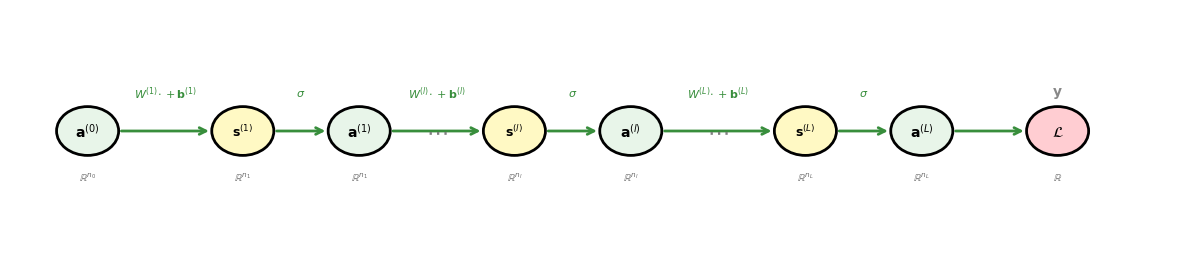
Per layer \(l = 1, \ldots, L\):
- \(\mathbf{s}^{(l)} = W^{(l)}\mathbf{a}^{(l-1)} + \mathbf{b}^{(l)}\) — pre-activation
- \(\mathbf{a}^{(l)} = \sigma(\mathbf{s}^{(l)})\) — activation (post-nonlinearity)
- \(W^{(l)} \in \mathbb{R}^{n_l \times n_{l-1}}\) — weight matrix
- \(\mathbf{b}^{(l)} \in \mathbb{R}^{n_l}\) — bias vector
- \(\sigma\) — activation function (sigmoid, ReLU, etc.)
Boundary and indexing:
- \(\mathbf{a}^{(0)} = \mathbf{x}\) — input (layer 0)
- \(\mathbf{a}^{(L)} = \hat{\mathbf{y}}\) — output (layer \(L\))
- \(\mathcal{L}(\hat{\mathbf{y}}, \mathbf{y})\) — loss (scalar)
- \(l\) indexes layers, \(L\) is the total count
Gradient shorthand:
- \(\boldsymbol{\delta}^{(l)} \equiv \frac{\partial \mathcal{L}}{\partial \mathbf{s}^{(l)}}\) — “delta” at layer \(l\)
Scalar Chain Rule
For \(y = f(g(x))\):
\[\frac{dy}{dx} = \frac{df}{dg} \cdot \frac{dg}{dx}\]
Example: \(y = \sigma(wx + b)\) with \(w=2, b=1, x=0.5\)
Forward:
\[z = 2(0.5) + 1 = 2\]
\[y = \sigma(2) = 0.881\]
Derivative:
\[\frac{dy}{dx} = \frac{dy}{dz} \cdot \frac{dz}{dx} = \sigma'(2) \cdot 2 = 0.881(1-0.881) \cdot 2 = 0.210\]
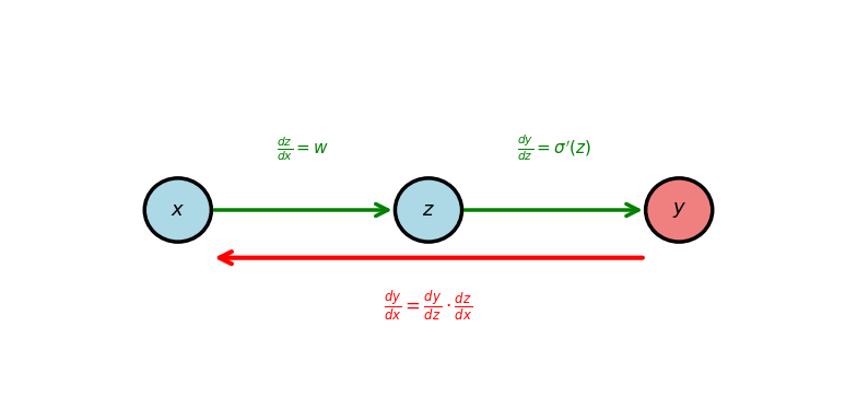
Chain rule: Multiply derivatives along path
Vector Chain Rule
For \(f: \mathbb{R}^m \to \mathbb{R}\) and \(\mathbf{y} = \mathbf{g}(\mathbf{x})\) where \(\mathbf{g}: \mathbb{R}^n \to \mathbb{R}^m\):
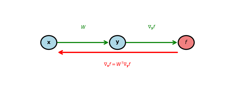
\[\frac{\partial f}{\partial x_i} = \sum_{j=1}^m \frac{\partial f}{\partial y_j} \frac{\partial y_j}{\partial x_i} \quad \Longleftrightarrow \quad \nabla_{\mathbf{x}} f = \left(\frac{\partial \mathbf{y}}{\partial \mathbf{x}}\right)^T \nabla_{\mathbf{y}} f\]
Jacobian \(\frac{\partial \mathbf{y}}{\partial \mathbf{x}} \in \mathbb{R}^{m \times n}\) transpose propagates gradients backward
Example: Composition \(g(\mathbf{y}(\mathbf{x}))\) where
- \(\mathbf{y} = W\mathbf{x}\) (linear transform)
- \(g(\mathbf{y}) = \mathbf{y}^T\mathbf{y}\) (squared norm)
\[W = \begin{bmatrix} 0.5 & 0.3 \\ -0.2 & 0.4 \end{bmatrix}, \quad \mathbf{x} = \begin{bmatrix} 1 \\ 2 \end{bmatrix}\]
Forward:
\[\mathbf{y} = \begin{bmatrix} 1.1 \\ 0.6 \end{bmatrix}, \quad g = 1.57\]
Gradient w.r.t. \(\mathbf{y}\):
\[\nabla_{\mathbf{y}} g = 2\mathbf{y} = \begin{bmatrix} 2.2 \\ 1.2 \end{bmatrix}\]
Gradient w.r.t. \(\mathbf{x}\) (via chain rule):
\[\nabla_{\mathbf{x}} g = W^T \nabla_{\mathbf{y}} g = \begin{bmatrix} 0.5 & -0.2 \\ 0.3 & 0.4 \end{bmatrix} \begin{bmatrix} 2.2 \\ 1.2 \end{bmatrix} = \begin{bmatrix} 0.86 \\ 1.14 \end{bmatrix}\]
Forward Pass Information Flow
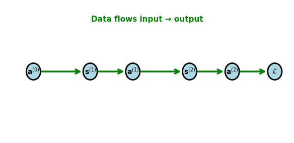
Forward computation:
Starting from \(\mathbf{a}^{(0)} = \mathbf{x}\):
For \(l = 1, 2, \ldots, L\):
\[\begin{align}
\mathbf{s}^{(l)} &= W^{(l)}\mathbf{a}^{(l-1)} + \mathbf{b}^{(l)}\\
\mathbf{a}^{(l)} &= \sigma^{(l)}(\mathbf{s}^{(l)})
\end{align}\]
Finally: \(\mathcal{L} = \mathcal{L}(\mathbf{a}^{(L)}, \mathbf{y})\)
Must store all \(\mathbf{a}^{(l)}\) and \(\mathbf{s}^{(l)}\) for backward pass:
- \(\mathbf{s}^{(l)}\) for activation derivatives
- \(\mathbf{a}^{(l-1)}\) for weight gradients
Storage requirement: \(O(\sum_{l=1}^L n_l)\) for all activations
Backward Pass Information Flow
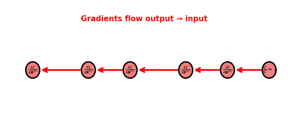
Backward computation:
Starting from \(\frac{\partial \mathcal{L}}{\partial \mathbf{a}^{(L)}}\):
For \(l = L, L-1, \ldots, 1\):
\[\begin{align}
\frac{\partial \mathcal{L}}{\partial \mathbf{s}^{(l)}} &= \frac{\partial \mathcal{L}}{\partial \mathbf{a}^{(l)}} \odot \sigma'^{(l)}(\mathbf{s}^{(l)})\\
\frac{\partial \mathcal{L}}{\partial W^{(l)}} &= \frac{\partial \mathcal{L}}{\partial \mathbf{s}^{(l)}} (\mathbf{a}^{(l-1)})^T\\
\frac{\partial \mathcal{L}}{\partial \mathbf{a}^{(l-1)}} &= (W^{(l)})^T \frac{\partial \mathcal{L}}{\partial \mathbf{s}^{(l)}}
\end{align}\]
Same graph, opposite direction
Complexity of backward ≈ Complexity of forward
Modular Layer Structure
Each layer implements two operations:
forward(input):
- Compute output from input
- Cache input and intermediate values
- Return output
backward(grad_output):
- Receive gradient w.r.t. output
- Compute gradient w.r.t. input
- Compute gradient w.r.t. parameters
- Return gradient w.r.t. input
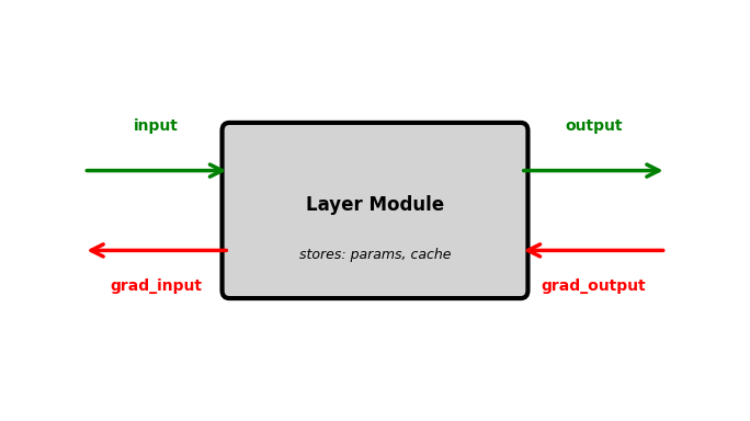
Example: Linear layer
class Linear:
    def forward(self, a_prev):
        self.a_prev = a_prev  # cache
        self.z = W @ a_prev + b
        return self.z

    def backward(self, grad_z):
        grad_W = grad_z @ a_prev.T
        grad_b = grad_z
        grad_a_prev = W.T @ grad_z
        return grad_a_prev
Example: Sigmoid layer
class Sigmoid:
    def forward(self, z):
        self.a = 1 / (1 + np.exp(-z))
        return self.a

    def backward(self, grad_a):
        grad_z = grad_a * self.a * (1 - self.a)
        return grad_z
Each module only needs its own inputs/outputs
No module needs global network structure
Backpropagation Overview
Network with \(L\) layers:
\(l \in \{1, 2, \ldots, L\}\), where \(\mathbf{s}^{(l)} = W^{(l)}\mathbf{a}^{(l-1)} + \mathbf{b}^{(l)}\) and \(\mathbf{a}^{(l)} = \sigma^{(l)}(\mathbf{s}^{(l)})\)
Boundary conditions:
- Input \(\mathbf{a}^{(0)} = \mathbf{x} \in \mathbb{R}^{n_0}\)
- Output \(\mathbf{a}^{(L)} = \hat{\mathbf{y}} \in \mathbb{R}^{n_L}\)
- Loss \(\mathcal{L} = \mathcal{L}(\hat{\mathbf{y}}, \mathbf{y})\)
Objective:
Compute \(\frac{\partial \mathcal{L}}{\partial W^{(l)}}\) and \(\frac{\partial \mathcal{L}}{\partial \mathbf{b}^{(l)}}\) for all \(l = 1, \ldots, L\) efficiently
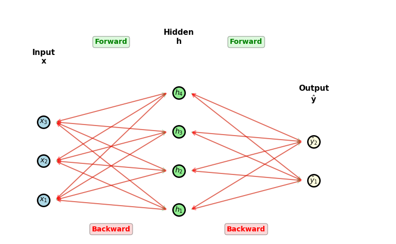
Forward: \(\mathbf{x} \xrightarrow{W^{(1)}} \mathbf{h} \xrightarrow{W^{(2)}} \hat{\mathbf{y}} \to \mathcal{L}\)
Store intermediate activations
Backward: \(\frac{\partial \mathcal{L}}{\partial W^{(1)}} \xleftarrow{} \frac{\partial \mathcal{L}}{\partial W^{(2)}} \xleftarrow{} \frac{\partial \mathcal{L}}{\partial \hat{\mathbf{y}}}\)
Update (\(\forall l = 1, \ldots, L\)):
\[W^{(l)} \leftarrow W^{(l)} - \eta \frac{\partial \mathcal{L}}{\partial W^{(l)}}\]
\[\mathbf{b}^{(l)} \leftarrow \mathbf{b}^{(l)} - \eta \frac{\partial \mathcal{L}}{\partial \mathbf{b}^{(l)}}\]
Dimensions: \(W^{(l)} \in \mathbb{R}^{n_l \times n_{l-1}}\), \(\mathbf{a}^{(l)}, \mathbf{s}^{(l)}, \mathbf{b}^{(l)} \in \mathbb{R}^{n_l}\)
Chain rule applied systematically from output to input
Scalar Two-Layer Network
Architecture: Two-layer scalar network
\[x \xrightarrow{w_1} s_1 \xrightarrow{\sigma} a_1 \xrightarrow{w_2} s_2 \xrightarrow{\sigma} \hat{y}\]
One scalar value per layer
Parameters:
- \(w_1 = 0.5\), \(b_1 = 0\)
- \(w_2 = -1\), \(b_2 = 0.5\)
Data:
- Input: \(x = 2\)
- Target: \(y = 1\)
Goal: Compute all gradients
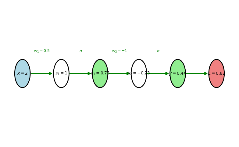
Forward values computed left to right
Forward Pass Computation
Layer 1:
\[s_1 = w_1 x + b_1 = 0.5(2) + 0 = 1\]
\[a_1 = \sigma(1) = \frac{1}{1+e^{-1}} = 0.731\]
Layer 2:
\[s_2 = w_2 a_1 + b_2 = -1(0.731) + 0.5 = -0.231\]
\[\hat{y} = \sigma(-0.231) = 0.442\]
Loss (binary cross-entropy, \(y=1\)):
\[\mathcal{L} = -\log(\hat{y}) = -\log(0.442) = 0.816\]
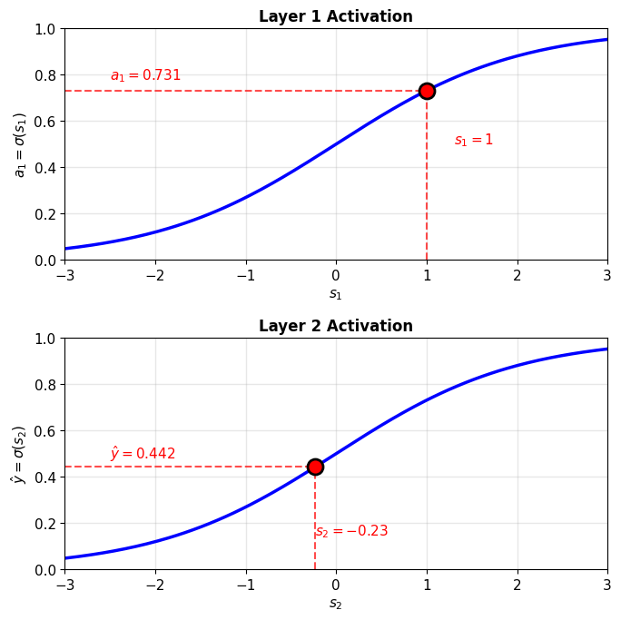
Sigmoid evaluation at specific pre-activation values
Backward Pass: Output Layer
Gradient w.r.t. \(\hat{y}\):
\[\frac{\partial \mathcal{L}}{\partial \hat{y}} = -\frac{y}{\hat{y}} + \frac{1-y}{1-\hat{y}} = -\frac{1}{0.442} = -2.262\]
Through sigmoid (\(\sigma'(z) = \sigma(z)(1-\sigma(z))\)):
\[\frac{\partial \hat{y}}{\partial s_2} = 0.442(1-0.442) = 0.247\]
Chain rule:
\[\frac{\partial \mathcal{L}}{\partial s_2} = -2.262 \times 0.247 = -0.558\]
Weight gradient:
\[\frac{\partial \mathcal{L}}{\partial w_2} = \frac{\partial \mathcal{L}}{\partial s_2} \times a_1 = -0.558 \times 0.731 = -0.408\]
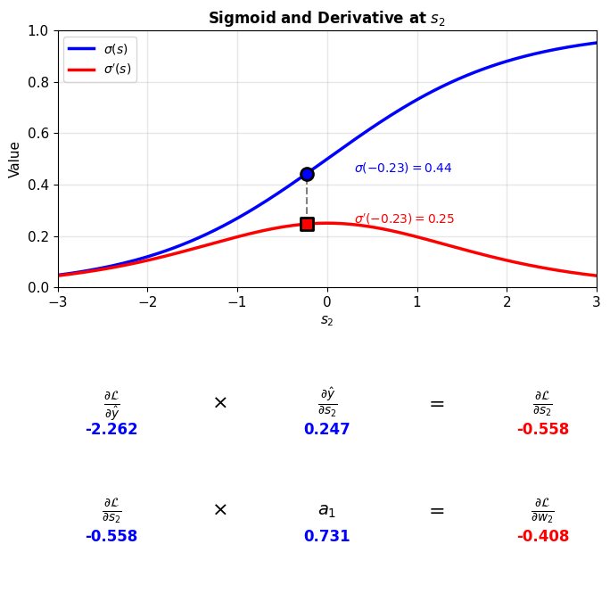
Delta: Gradient w.r.t. Pre-Activation
Define: \(\delta^{(l)} \equiv \frac{\partial \mathcal{L}}{\partial s^{(l)}}\) (gradient w.r.t. pre-activation)
Why useful: Appears repeatedly in gradient computation
For our network:
Output layer:
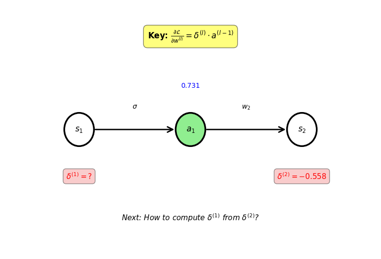
\[\delta^{(2)} = \frac{\partial \mathcal{L}}{\partial s_2} = -0.558\]
Hidden layer:
\[\delta^{(1)} = \frac{\partial \mathcal{L}}{\partial s_1} = ?\]
Weight gradients simplify:
\[\frac{\partial \mathcal{L}}{\partial w_2} = \delta^{(2)} \cdot a_1 = -0.558 \times 0.731 = -0.408\]
\[\frac{\partial \mathcal{L}}{\partial b_2} = \delta^{(2)} = -0.558\]
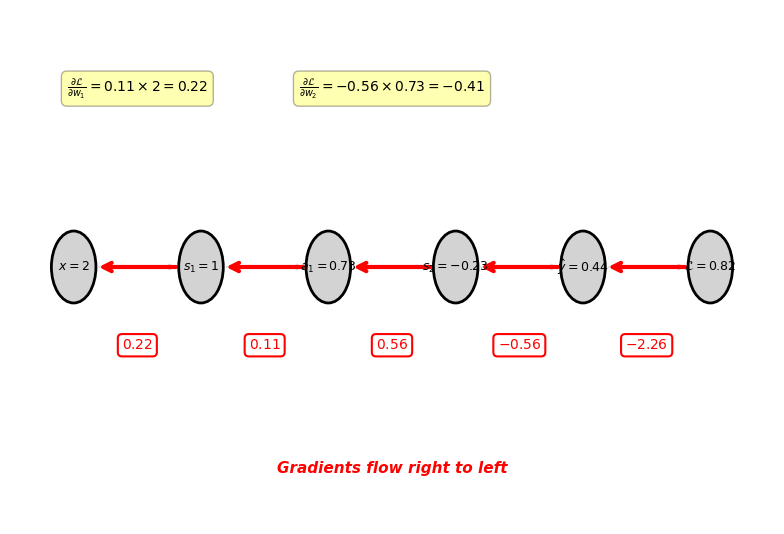
Backpropagation Flow: Scalar Network
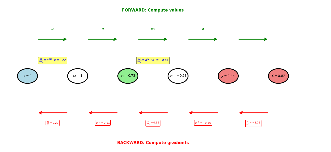
Forward pass computes values, backward pass computes gradients using chain rule
Network with Branching
Architecture: Two hidden units
\[x \to \begin{cases} h_1 = \sigma(w_1 x + b_1) \\ h_2 = \sigma(w_2 x + b_2) \end{cases} \to y = w_3 h_1 + w_4 h_2\]
Parameters: \(w_1 = 0.5, w_2 = -0.3, w_3 = 1, w_4 = 1\), all biases zero
Data: \(x = 1\), target \(t = 0.5\)
Forward:
\(h_1 = \sigma(0.5) = 0.622\)
\(h_2 = \sigma(-0.3) = 0.426\)
\(y = 0.622 + 0.426 = 1.048\)
Loss: \(\mathcal{L} = \frac{1}{2}(1.048 - 0.5)^2 = 0.150\)
Backward: \(\frac{\partial \mathcal{L}}{\partial y} = 1.048 - 0.5 = 0.548\)
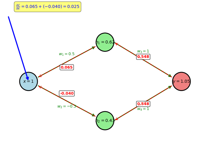
Multiple gradient paths converge at \(x\)
Gradient Accumulation Rule
Multivariate chain rule:
Two paths from \(\mathcal{L}\) to \(x\):
\[\frac{\partial \mathcal{L}}{\partial x} = \frac{\partial \mathcal{L}}{\partial h_1}\frac{\partial h_1}{\partial x} + \frac{\partial \mathcal{L}}{\partial h_2}\frac{\partial h_2}{\partial x}\]
Path 1 contribution:
\[\frac{\partial \mathcal{L}}{\partial y} = y - t = 1.048 - 0.5 = 0.548\]
\[\frac{\partial \mathcal{L}}{\partial h_1} = \frac{\partial \mathcal{L}}{\partial y} \cdot \frac{\partial y}{\partial h_1} = 0.548 \cdot w_3 = 0.548 \cdot 1 = 0.548\]
\[\frac{\partial h_1}{\partial x} = \sigma'(w_1 x) \cdot w_1 = 0.622(0.378) \cdot 0.5 = 0.118\]
\[\text{Contribution}_1 = 0.548 \cdot 0.118 = 0.065\]
Path 2 contribution:
\[\frac{\partial \mathcal{L}}{\partial h_2} = \frac{\partial \mathcal{L}}{\partial y} \cdot \frac{\partial y}{\partial h_2} = 0.548 \cdot w_4 = 0.548 \cdot 1 = 0.548\]
\[\frac{\partial h_2}{\partial x} = \sigma'(w_2 x) \cdot w_2 = 0.426(0.574) \cdot (-0.3) = -0.073\]
\[\text{Contribution}_2 = 0.548 \cdot (-0.073) = -0.040\]
Total gradient:
\[\frac{\partial \mathcal{L}}{\partial x} = 0.065 + (-0.040) = 0.025\]
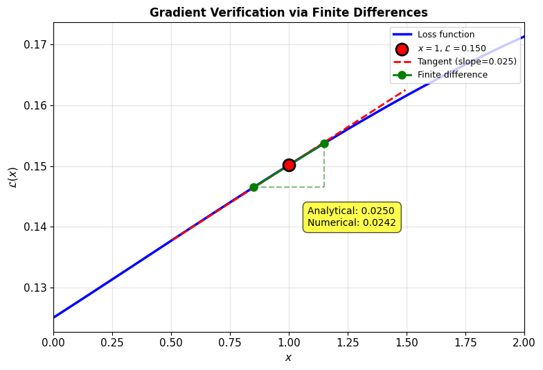
Analytical gradient matches numerical
When multiple paths converge, gradients add
Delta Recursion: 3-Layer Network
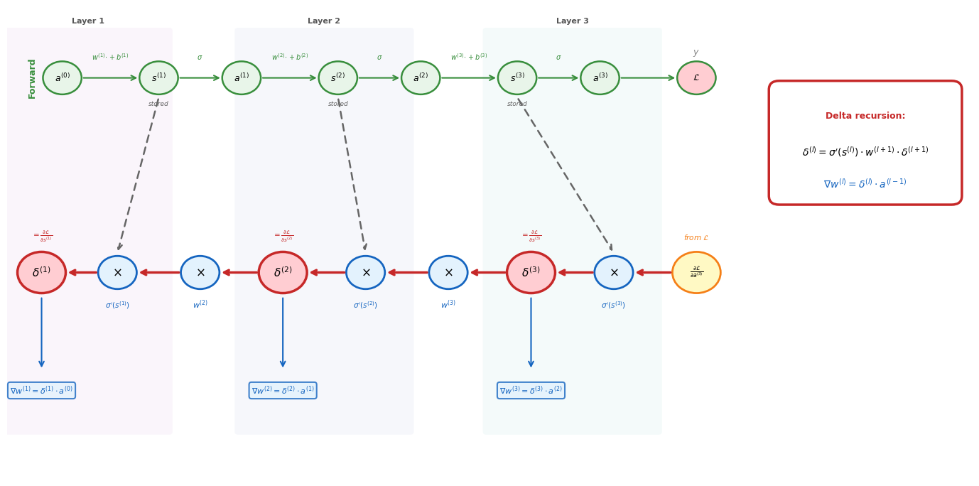
Each \(\delta^{(l)}\) requires two multiplications: \(\sigma'(s^{(l)})\) (uses stored pre-activation) and \(w^{(l+1)}\) (upstream weight). Weight gradients branch off each delta.
Two-Layer Network Architecture
Scalar to vector: Binary classification (1 output) → Multi-class classification (K outputs)
Sigmoid: \(\hat{y} = \sigma(s) \in (0,1)\) (probability of class 1)
Softmax: \(\hat{\mathbf{y}} = \text{softmax}(\mathbf{s}) \in \mathbb{R}^K\), \(\sum_i \hat{y}_i = 1\) (probability distribution over K classes)
Dimensions:
- Input: \(\mathbf{x} \in \mathbb{R}^3\)
- Hidden: \(\mathbf{h} \in \mathbb{R}^4\)
- Output: \(\mathbf{y} \in \mathbb{R}^2\) (2-class example)
Parameters:
Layer 1:
- \(W^{(1)} \in \mathbb{R}^{4 \times 3}\): 12 weights
- \(\mathbf{b}^{(1)} \in \mathbb{R}^4\): 4 biases
Layer 2:
- \(W^{(2)} \in \mathbb{R}^{2 \times 4}\): 8 weights
- \(\mathbf{b}^{(2)} \in \mathbb{R}^2\): 2 biases
Total: 26 parameters
Forward pass:
\[\mathbf{s}^{(1)} = W^{(1)}\mathbf{x} + \mathbf{b}^{(1)}, \quad \mathbf{a}^{(1)} = \sigma(\mathbf{s}^{(1)})\]
\[\mathbf{s}^{(2)} = W^{(2)}\mathbf{a}^{(1)} + \mathbf{b}^{(2)}, \quad \mathbf{a}^{(2)} = \text{softmax}(\mathbf{s}^{(2)})\]
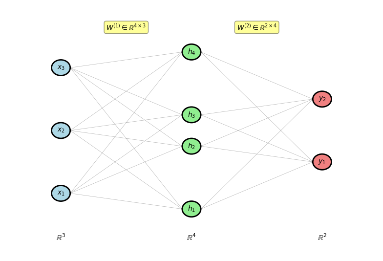
Fully connected: every unit in one layer connects to every unit in next layer
Jacobian: Dense for Linear, Diagonal for Activation
Jacobian matrix: All partial derivatives
For \(\mathbf{y} = f(\mathbf{x})\) where \(\mathbf{y} \in \mathbb{R}^m\), \(\mathbf{x} \in \mathbb{R}^n\):
\[J = \frac{\partial \mathbf{y}}{\partial \mathbf{x}} = \begin{bmatrix}
\frac{\partial y_1}{\partial x_1} & \cdots & \frac{\partial y_1}{\partial x_n} \\
\vdots & \ddots & \vdots \\
\frac{\partial y_m}{\partial x_1} & \cdots & \frac{\partial y_m}{\partial x_n}
\end{bmatrix} \in \mathbb{R}^{m \times n}\]
Linear layer:
\[\mathbf{s} = W\mathbf{a} + \mathbf{b}\]
\[\frac{\partial \mathbf{s}}{\partial \mathbf{a}} = W\]
Element-wise activation:
\[a_i = \sigma(s_i)\]
\[\frac{\partial \mathbf{a}}{\partial \mathbf{s}} = \text{diag}(\sigma'(s_1), \ldots, \sigma'(s_n))\]
Diagonal because \(\frac{\partial a_i}{\partial s_j} = 0\) for \(i \neq j\)
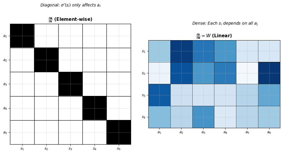
Jacobian structure reflects dependencies
Hadamard Product Simplifies Diagonal Matrix Multiply
Hadamard product (element-wise multiply): \(\odot\)
\[\mathbf{a} \odot \mathbf{b} = \begin{bmatrix} a_1 b_1 \\ a_2 b_2 \\ \vdots \\ a_n b_n \end{bmatrix}\]
Example:
\[\begin{bmatrix} 2 \\ 3 \\ -1 \end{bmatrix} \odot \begin{bmatrix} 0.5 \\ 0.2 \\ 0.8 \end{bmatrix} = \begin{bmatrix} 1.0 \\ 0.6 \\ -0.8 \end{bmatrix}\]
Connection to diagonal matrix:
\[\text{diag}(\mathbf{a} \odot \mathbf{b}) = \text{diag}(\mathbf{a}) \text{diag}(\mathbf{b})\]
\[\mathbf{a} \odot \mathbf{b} = \text{diag}(\mathbf{a}) \mathbf{b} = \text{diag}(\mathbf{b}) \mathbf{a}\]
where \(\text{diag}(\mathbf{a})\) puts vector on diagonal:
\[\text{diag}([a_1, a_2, a_3]^T) = \begin{bmatrix} a_1 & 0 & 0 \\ 0 & a_2 & 0 \\ 0 & 0 & a_3 \end{bmatrix}\]
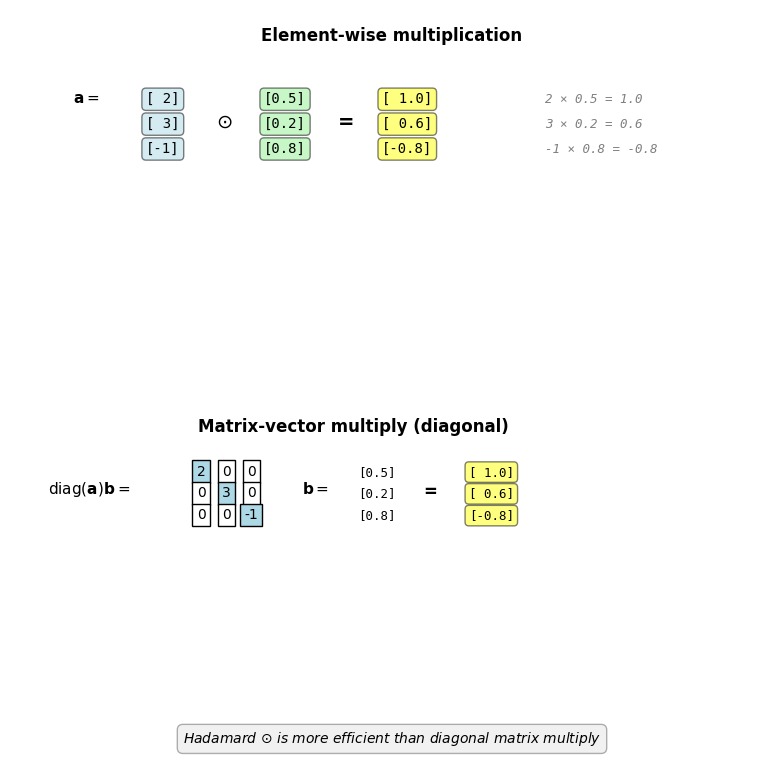
Used in backprop to apply element-wise activation derivatives
Backpropagation Flow: Vector Network
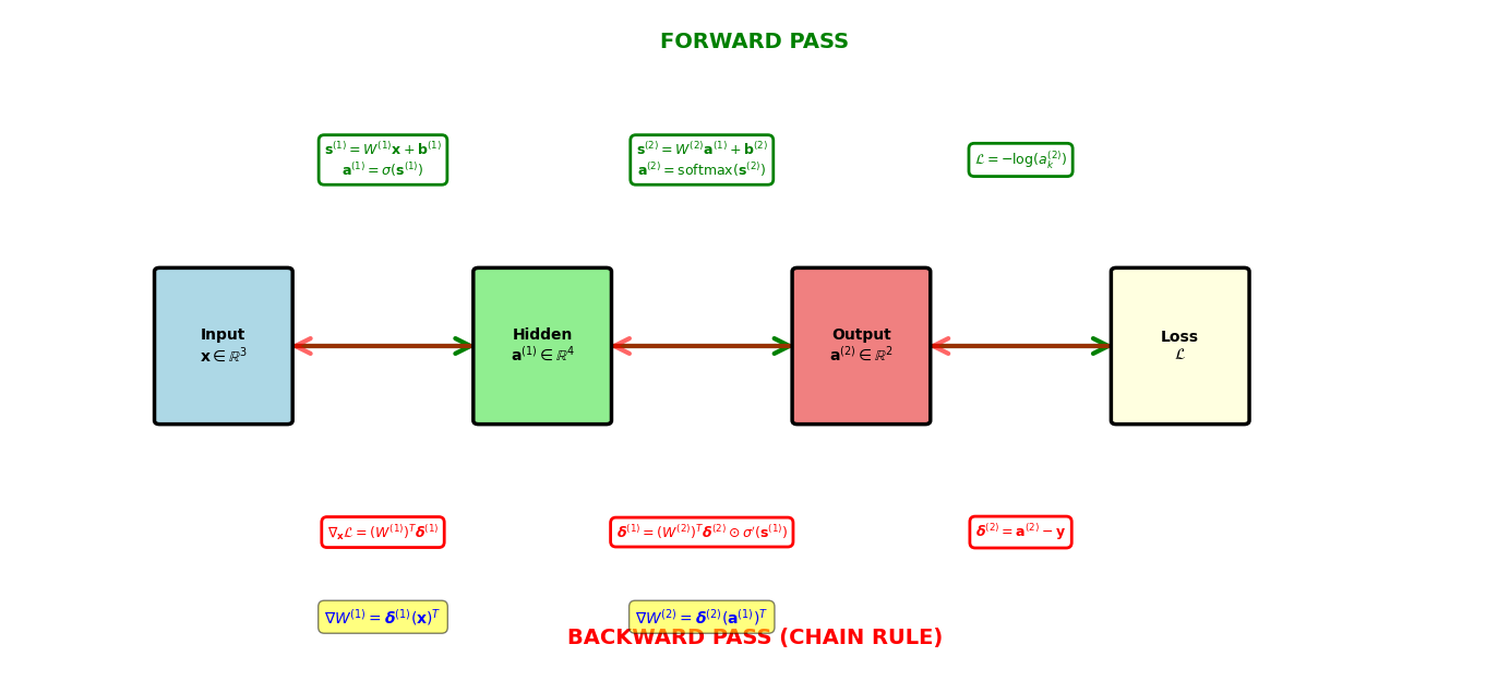
Delta propagates backward, weight gradients computed via outer products
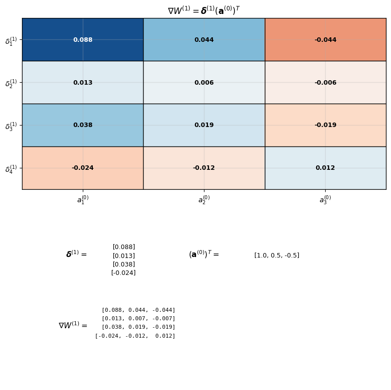
Weight Gradient as Outer Product
Scalar to matrix derivation:
Layer computation: \(s_i^{(l)} = \sum_{j=1}^{n_{l-1}} w_{ij}^{(l)} a_j^{(l-1)} + b_i^{(l)}\)
Chain rule:
\[\frac{\partial \mathcal{L}}{\partial w_{ij}^{(l)}} = \frac{\partial \mathcal{L}}{\partial s_i^{(l)}} \cdot \frac{\partial s_i^{(l)}}{\partial w_{ij}^{(l)}} = \delta_i^{(l)} \cdot a_j^{(l-1)}\]
Matrix form (all elements):
\[\left[\frac{\partial \mathcal{L}}{\partial W^{(l)}}\right]_{ij} = \delta_i^{(l)} \cdot a_j^{(l-1)}\]
Recognize outer product:
\[\frac{\partial \mathcal{L}}{\partial W^{(l)}} = \boldsymbol{\delta}^{(l)} (\mathbf{a}^{(l-1)})^T\]
Dimensions: \([n_l \times 1][1 \times n_{l-1}] = [n_l \times n_{l-1}]\) ✓
Bias gradient:
\[\frac{\partial \mathcal{L}}{\partial \mathbf{b}^{(l)}} = \boldsymbol{\delta}^{(l)}\]
Backpropagation Algorithm
Input: Network \(\{W^{(l)}, \mathbf{b}^{(l)}\}_{l=1}^L\), data \((\mathbf{x}, \mathbf{y})\)
Output: Gradients \(\{\nabla W^{(l)}, \nabla \mathbf{b}^{(l)}\}_{l=1}^L\)
Forward pass:
a⁽⁰⁾ ← x
for l = 1 to L:
  s⁽ˡ⁾ ← W⁽ˡ⁾ a⁽ˡ⁻¹⁾ + b⁽ˡ⁾
  a⁽ˡ⁾ ← σ⁽ˡ⁾(s⁽ˡ⁾)
  store: a⁽ˡ⁻¹⁾, s⁽ˡ⁾, a⁽ˡ⁾
Backward pass:
δ⁽ᴸ⁾ ← ∇_a⁽ᴸ⁾ 𝓛(a⁽ᴸ⁾, y)
for l = L down to 1:
  δ⁽ˡ⁾ ← (W⁽ˡ⁺¹⁾)ᵀ δ⁽ˡ⁺¹⁾ ⊙ σ'(s⁽ˡ⁾)
Gradient computation:
for l = 1 to L:
  ∇W⁽ˡ⁾ ← δ⁽ˡ⁾ (a⁽ˡ⁻¹⁾)ᵀ
  ∇b⁽ˡ⁾ ← δ⁽ˡ⁾
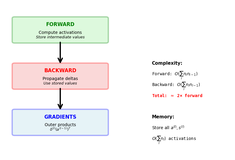
Single forward pass + single backward pass computes all gradients
Activation Function Derivatives
Algorithm unchanged—only \(\sigma'(\mathbf{s}^{(l)})\) differs per layer
Sigmoid: \(\sigma(s) = \frac{1}{1+e^{-s}}\)
\[\sigma'(s) = \sigma(s)(1-\sigma(s))\]
Can compute from stored activation: \(a(1-a)\)
Tanh: \(\sigma(s) = \tanh(s)\)
\[\tanh'(s) = 1 - \tanh^2(s)\]
Also from activation: \(1 - a^2\)
ReLU: \(\sigma(s) = \max(0, s)\)
\[\text{ReLU}'(s) = \begin{cases} 1 & s > 0 \\ 0 & s \leq 0 \end{cases}\]
Indicator function (discontinuous at 0)
Leaky ReLU: \(\sigma(s) = \max(\alpha s, s)\) with \(\alpha = 0.01\)
\[\text{LReLU}'(s) = \begin{cases} 1 & s > 0 \\ \alpha & s \leq 0 \end{cases}\]
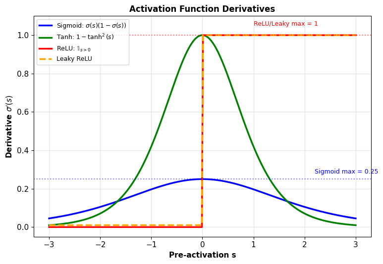
ReLU advantages:
- Sparse gradients (50% zeros)
- No vanishing gradient for active units (\(s > 0\))
- Cheap to compute
Backprop Scales: 244K Gradients in Two Passes
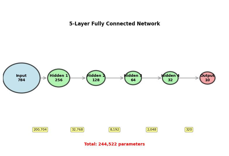
Architecture: MNIST digit classifier
\[784 \to 256 \to 128 \to 64 \to 32 \to 10\]
Input: 28×28 grayscale images = 784 pixels
Output: 10 class probabilities
Parameters per layer:
- \(W^{(1)}\): \(256 \times 784 = 200{,}704\)
- \(W^{(2)}\): \(128 \times 256 = 32{,}768\)
- \(W^{(3)}\): \(64 \times 128 = 8{,}192\)
- \(W^{(4)}\): \(32 \times 64 = 2{,}048\)
- \(W^{(5)}\): \(10 \times 32 = 320\)
Biases: \(256 + 128 + 64 + 32 + 10 = 490\)
Total: \(244{,}032\) weights + \(490\) biases = \(244{,}522\) parameters
Backprop computes all 244,522 gradients in 2 passes (1 forward + 1 backward)
Gradient Flow Through Depth
Delta magnitude at layer \(l\):
\[\|\boldsymbol{\delta}^{(l)}\| \approx \|\boldsymbol{\delta}^{(L)}\| \prod_{k=l+1}^L \|W^{(k)}\| \|\sigma'(\mathbf{s}^{(k)})\|\]
Rough approximation ignoring vector structure
Sigmoid network:
Maximum derivative: \(\max_s \sigma'(s) = 0.25\) at \(s=0\)
Typical values: \(\sigma'(s) \approx 0.2\) in practice
After 10 layers: \((0.2)^{10} \approx 10^{-7}\)
Gradients vanish exponentially with depth
Early layers receive near-zero gradients, fail to train
ReLU network:
Derivative: \(\text{ReLU}'(s) \in \{0, 1\}\)
Active units (\(s > 0\)): gradient = 1 (no shrinking)
Dead units (\(s \leq 0\)): gradient = 0 (propagation stops)
Better gradient flow if units stay active
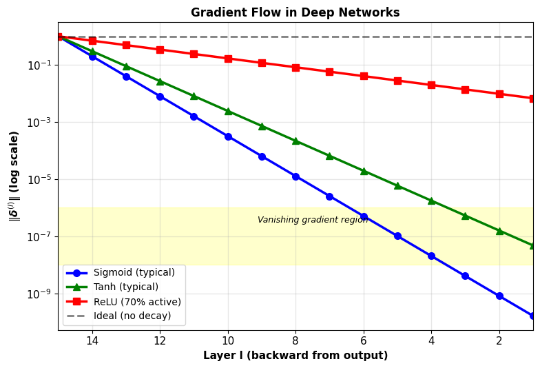
Sigmoid/tanh: Exponential decay
ReLU: Better but still degrades
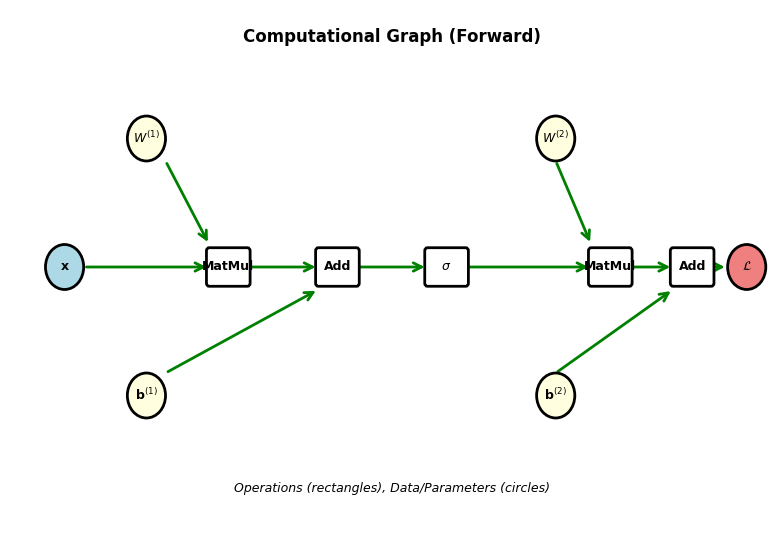
Networks as Directed Acyclic Graphs
Nodes: Operations (MatMul, Add, Sigmoid, etc.)
Edges: Tensors flowing between operations
Example: 2-layer network decomposed
Forward: \(\mathbf{x} \to W^{(1)}\mathbf{x} \to + \mathbf{b}^{(1)} \to \sigma \to W^{(2)} \to + \mathbf{b}^{(2)} \to \sigma \to \mathcal{L}\)
Each arrow represents data dependency
Directed: Information flows one direction (forward)
Acyclic: No loops (feedforward network)
Topological order: Can order nodes so all inputs come before outputs
Forward pass: Traverse in topological order
Backward pass: Traverse in reverse topological order
Benefits:
- Modular: Each operation self-contained
- Composable: Build complex functions from primitives
- Automatic: Can differentiate any graph mechanically
Local Gradient Principle
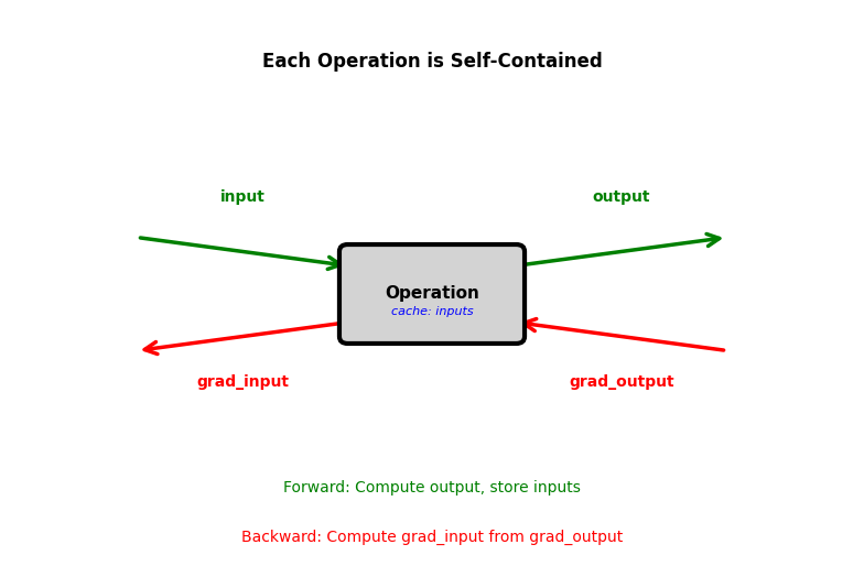
Each node: Implements forward and backward
class Operation:
    def forward(self, inputs):
        # Compute output from inputs
        # Cache inputs for backward
        self.cache = inputs
        return self.compute(inputs)

    def backward(self, grad_output):
        # Compute gradient w.r.t. inputs
        # Use cached values
        return self.local_gradient(
            grad_output, self.cache)
No global knowledge required
Node only needs:
- How to compute output from inputs (forward)
- How to compute input gradients from output gradient (backward)
Chain rule automatic:
Graph framework connects local gradients
Node A → Node B: \(\frac{\partial \mathcal{L}}{\partial \text{input}_A} = \frac{\partial \text{output}_B}{\partial \text{input}_A}^T \frac{\partial \mathcal{L}}{\partial \text{output}_B}\)
Framework handles composition
Matrix Multiplication Node
Forward: \(\mathbf{y} = A\mathbf{x}\)
Input: Matrix \(A \in \mathbb{R}^{m \times n}\), vector \(\mathbf{x} \in \mathbb{R}^n\)
Output: \(\mathbf{y} \in \mathbb{R}^m\)
Backward: Given \(\frac{\partial \mathcal{L}}{\partial \mathbf{y}}\), compute gradients w.r.t. inputs
Gradient w.r.t. \(\mathbf{x}\):
\[\frac{\partial \mathcal{L}}{\partial \mathbf{x}} = A^T \frac{\partial \mathcal{L}}{\partial \mathbf{y}}\]
Dimension: \([n \times 1] = [n \times m][m \times 1]\)
Gradient w.r.t. \(A\):
\[\frac{\partial \mathcal{L}}{\partial A} = \frac{\partial \mathcal{L}}{\partial \mathbf{y}} \mathbf{x}^T\]
Dimension: \([m \times n] = [m \times 1][1 \times n]\)
Implementation:
class MatMul:
    def forward(self, A, x):
        self.A, self.x = A, x
        return A @ x

    def backward(self, grad_y):
        grad_x = self.A.T @ grad_y
        grad_A = np.outer(grad_y, self.x)
        return grad_A, grad_x
Numerical example:
\[A = \begin{bmatrix} 0.5 & 0.3 \\ -0.2 & 0.4 \end{bmatrix}, \quad \mathbf{x} = \begin{bmatrix} 1 \\ 2 \end{bmatrix}\]
Forward:
\[\mathbf{y} = \begin{bmatrix} 0.5(1) + 0.3(2) \\ -0.2(1) + 0.4(2) \end{bmatrix} = \begin{bmatrix} 1.1 \\ 0.6 \end{bmatrix}\]
Backward (assume \(\frac{\partial \mathcal{L}}{\partial \mathbf{y}} = \begin{bmatrix} 0.8 \\ -0.5 \end{bmatrix}\)):
\[\frac{\partial \mathcal{L}}{\partial \mathbf{x}} = \begin{bmatrix} 0.5 & -0.2 \\ 0.3 & 0.4 \end{bmatrix} \begin{bmatrix} 0.8 \\ -0.5 \end{bmatrix} = \begin{bmatrix} 0.5 \\ 0.04 \end{bmatrix}\]
\[\frac{\partial \mathcal{L}}{\partial A} = \begin{bmatrix} 0.8 \\ -0.5 \end{bmatrix} \begin{bmatrix} 1 & 2 \end{bmatrix} = \begin{bmatrix} 0.8 & 1.6 \\ -0.5 & -1.0 \end{bmatrix}\]

Addition Node
Forward: \(z = x + y\)
Inputs: Scalars, vectors, or matrices (same shape)
Output: Same shape as inputs
Backward: Given \(\frac{\partial \mathcal{L}}{\partial z}\)
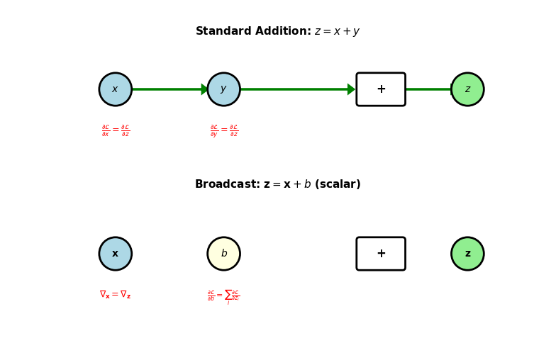
Addition distributes gradient to both inputs:
\[\frac{\partial \mathcal{L}}{\partial x} = \frac{\partial \mathcal{L}}{\partial z}\]
\[\frac{\partial \mathcal{L}}{\partial y} = \frac{\partial \mathcal{L}}{\partial z}\]
Gradient copies to each input (no modification)
Broadcast addition: \(\mathbf{z} = \mathbf{x} + b\) where \(b\) scalar
Forward: Add \(b\) to each element of \(\mathbf{x}\)
Backward:
\[\frac{\partial \mathcal{L}}{\partial \mathbf{x}} = \frac{\partial \mathcal{L}}{\partial \mathbf{z}}\]
\[\frac{\partial \mathcal{L}}{\partial b} = \sum_i \frac{\partial \mathcal{L}}{\partial z_i}\]
Gradient w.r.t. scalar sums gradients from all elements
Gradient distribution rule:
- Fork (1→many): Copy gradient
- Join (many→1): Sum gradients
Element-Wise Activation Node
Forward: \(\mathbf{a} = \sigma(\mathbf{s})\)
Apply function element-wise: \(a_i = \sigma(s_i)\)
Backward: Given \(\frac{\partial \mathcal{L}}{\partial \mathbf{a}}\)
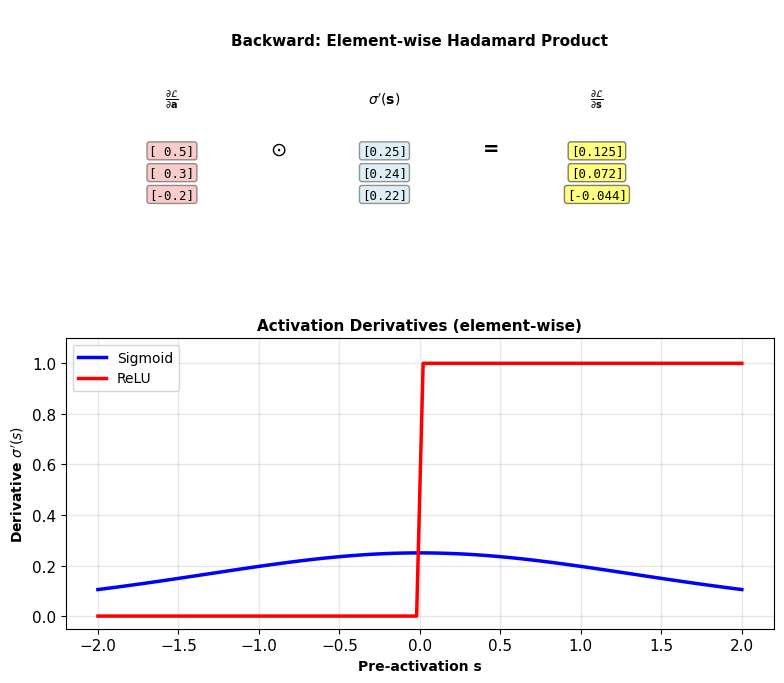
\[\frac{\partial \mathcal{L}}{\partial \mathbf{s}} = \frac{\partial \mathcal{L}}{\partial \mathbf{a}} \odot \sigma'(\mathbf{s})\]
Hadamard product (element-wise multiply)
Each \(\frac{\partial \mathcal{L}}{\partial s_i} = \frac{\partial \mathcal{L}}{\partial a_i} \cdot \sigma'(s_i)\)
Different activations:
Sigmoid: \(\sigma'(s) = \sigma(s)(1-\sigma(s))\) (can compute from \(a\))
ReLU: \(\sigma'(s) = \mathbb{1}_{s > 0}\) (needs \(s\), not just \(a\))
Implementation:
class Sigmoid:
    def forward(self, s):
        self.a = 1 / (1 + np.exp(-s))
        return self.a

    def backward(self, grad_a):
        # Use cached activation
        grad_s = grad_a * self.a * (1 - self.a)
        return grad_s
Multiple Paths: Fork and Join
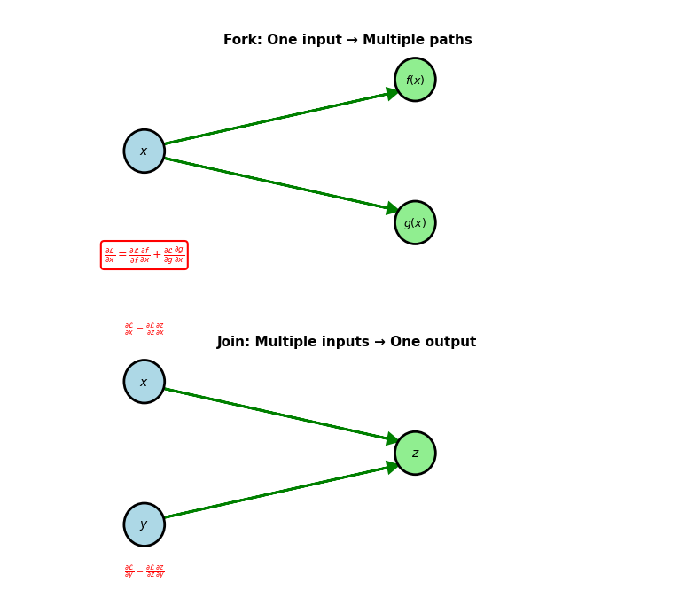
Fork (one input, multiple outputs):
Single value used by multiple operations
Example: \(x \to f(x)\) and \(x \to g(x)\)
Backward: Gradients from all paths sum
\[\frac{\partial \mathcal{L}}{\partial x} = \frac{\partial \mathcal{L}}{\partial f} \frac{\partial f}{\partial x} + \frac{\partial \mathcal{L}}{\partial g} \frac{\partial g}{\partial x}\]
Each path contributes independently
Join (multiple inputs, one output):
Multiple values combine into single operation
Example: \(z = f(x, y)\)
Backward: Each input gets its gradient
\[\frac{\partial \mathcal{L}}{\partial x} = \frac{\partial \mathcal{L}}{\partial z} \frac{\partial z}{\partial x}\]
\[\frac{\partial \mathcal{L}}{\partial y} = \frac{\partial \mathcal{L}}{\partial z} \frac{\partial z}{\partial y}\]
Separate gradients for each input
Skip connections, attention mechanisms: Multiple paths converge
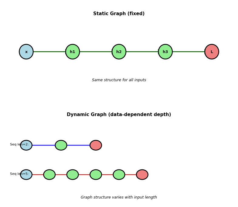
Dynamic Graphs Build Structure at Runtime
Static graph: Structure fixed before execution
Build graph once, execute many times
TensorFlow 1.x, compiled frameworks
Optimization possible (graph fusion, memory planning)
Cannot change based on data
Dynamic graph: Structure built during forward pass
Graph structure can depend on data
PyTorch, TensorFlow 2.x (eager mode)
Example: Variable-length sequences
RNN processing sentence: Graph depth = sequence length
Different inputs \(\to\) different graphs
Backward pass: Follow actual graph from forward
Only differentiate paths that were executed
Benefits:
- Control flow (if/while in forward)
- Data-dependent architecture
- Easier debugging (standard Python)
Cost: Less optimization opportunity
Two-Layer Network in NumPy
import numpy as np

class TwoLayerNet:
    def __init__(self, input_dim, hidden_dim,
                 output_dim):
        # Xavier initialization
        self.W1 = np.random.randn(
            hidden_dim, input_dim
        ) * np.sqrt(2 / input_dim)
        self.b1 = np.zeros(hidden_dim)

        self.W2 = np.random.randn(
            output_dim, hidden_dim
        ) * np.sqrt(2 / hidden_dim)
        self.b2 = np.zeros(output_dim)

        # Store forward pass values
        self.cache = {}
Example: 784 → 256 → 10 network
net = TwoLayerNet(
    input_dim=784,    # MNIST images
    hidden_dim=256,   # Hidden units
    output_dim=10     # Digit classes
)

# Parameters
# W1: 256 × 784 = 200,704
# b1: 256
# W2: 10 × 256 = 2,560
# b2: 10
# Total: 203,530 parameters
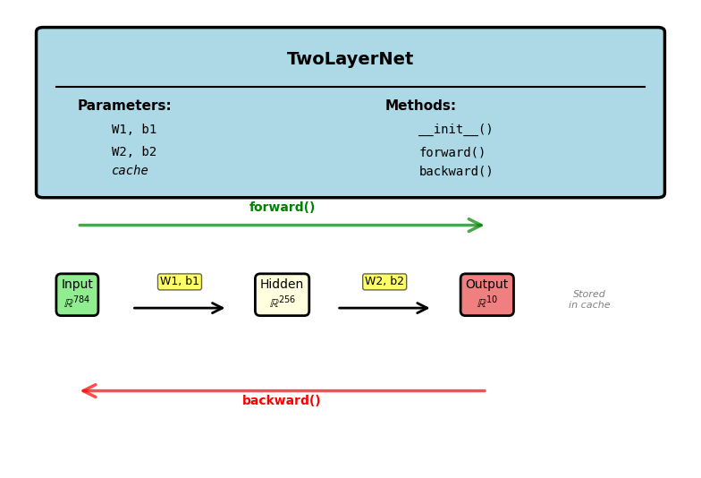
Forward-Backward-Update: Training Loop
# Generate synthetic data
np.random.seed(42)
n_samples = 1000
n_features = 20
n_classes = 5

# Random features
X = np.random.randn(n_samples, n_features)

# Random labels (one-hot)
labels = np.random.randint(0, n_classes,
                           n_samples)
y = np.zeros((n_samples, n_classes))
y[np.arange(n_samples), labels] = 1

# Initialize network
net = TwoLayerNet(
    input_dim=n_features,
    hidden_dim=50,
    output_dim=n_classes
)

# Train
losses = []
for epoch in range(500):
    # Forward
    predictions = net.forward(X)
    loss = -np.mean(np.sum(
        y * np.log(predictions + 1e-10),
        axis=1
    ))
    losses.append(loss)

    # Backward
    net.backward(y)

    # Update
    net.update_parameters(learning_rate=0.1)
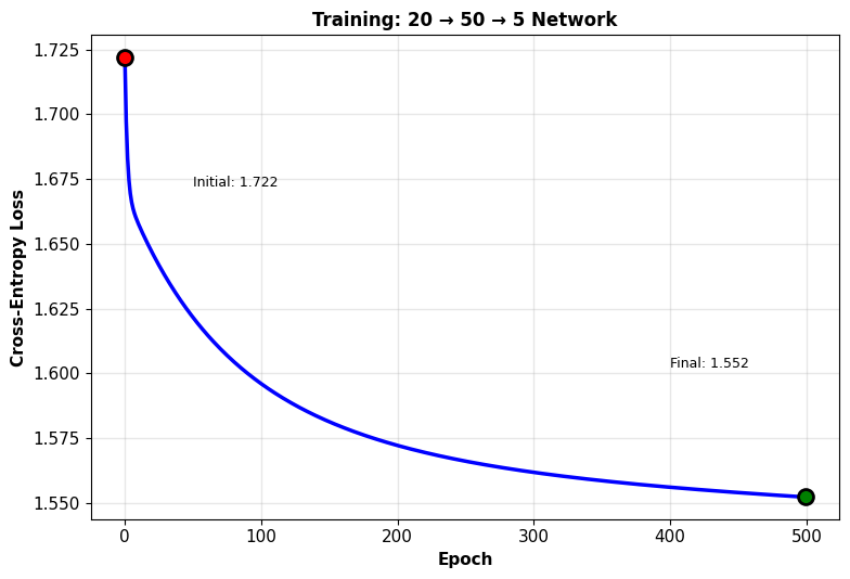
Loss: \(1.609 \to 1.456\) (random labels, cannot fit perfectly)
Gradient Verification
Finite difference approximation:
\[\frac{\partial \mathcal{L}}{\partial w} \approx \frac{\mathcal{L}(w + \epsilon) - \mathcal{L}(w - \epsilon)}{2\epsilon}\]
Centered difference: \(O(\epsilon^2)\) error
Choice of \(\epsilon\): \(10^{-5}\) to \(10^{-7}\)
Too large: truncation error from Taylor expansion
Too small: numerical cancellation (roundoff error)
Implementation:
def gradient_check(net, X, y, eps=1e-5):
    # Analytical gradient
    net.forward(X)
    net.backward(y)
    analytic = net.dW1.copy()

    # Numerical gradient
    def loss_fn(W):
        net.W1 = W.reshape(net.W1.shape)
        pred = net.forward(X)
        return -np.mean(np.sum(
            y * np.log(pred + 1e-10), axis=1
        ))

    W_flat = net.W1.flatten()
    numeric = numerical_gradient(
        loss_fn, W_flat, eps
    ).reshape(net.W1.shape)

    # Relative error
    diff = np.linalg.norm(analytic - numeric)
    scale = np.linalg.norm(analytic) + \
            np.linalg.norm(numeric)
    return diff / scale
Relative error metric:
\[\text{error} = \frac{\|\nabla_{\text{analytic}} - \nabla_{\text{numeric}}\|}{\|\nabla_{\text{analytic}}\| + \|\nabla_{\text{numeric}}\|}\]
Scale-invariant comparison
Thresholds:
- \(< 10^{-7}\): Implementation correct
- \(10^{-7}\) to \(10^{-5}\): Acceptable (check carefully)
- \(> 10^{-5}\): Bug in implementation
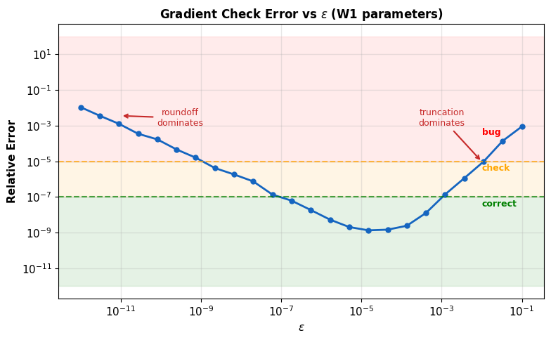
Sweet spot at \(\epsilon \approx 10^{-5}\) to \(10^{-7}\): U-shaped curve from competing error sources
When Gradient Check Fails
Buggy implementation: Missing sigmoid derivative
def backward_buggy(self, y_true):
    m = y_true.shape[0]

    delta2 = (self.cache['A2'] - y_true) / m
    self.dW2 = delta2.T @ self.cache['A1']
    self.db2 = np.sum(delta2, axis=0)

    # BUG: Missing activation derivative
    delta1 = (delta2 @ self.W2)  # Wrong!
    # Should be:
    # delta1 = (delta2 @ self.W2) * A1 * (1-A1)

    self.dW1 = delta1.T @ self.cache['A0']
    self.db1 = np.sum(delta1, axis=0)
Gradient check result:
error = gradient_check(buggy_net, X, y)
print(f"Relative error: {error:.2e}")
# Output: Relative error: 7.34e-01
Error \(\sim 0.7\): Implementation wrong
Correct implementation: Error < \(10^{-7}\)
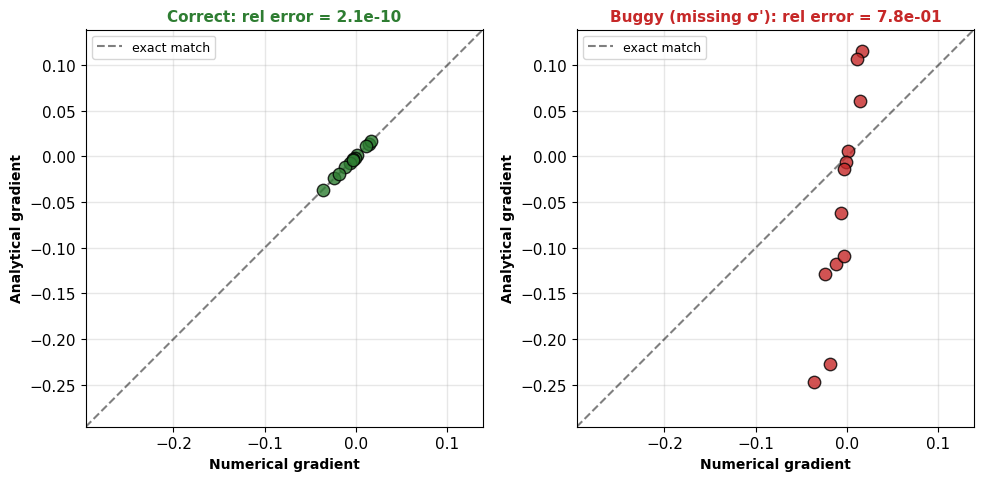
Correct: points on diagonal. Buggy: systematic deviation — missing \(\sigma'\) distorts every gradient element
Memory Cost: Parameters, Gradients, and Activations
784→256→128→10, float32 (4 bytes per value)
Parameters (fixed, independent of batch):
\(W^{(1)}\): \(256 \times 784 = 200{,}704\) values → 803 KB
\(W^{(2)}\): \(128 \times 256 = 32{,}768\) values → 131 KB
\(W^{(3)}\): \(10 \times 128 = 1{,}280\) values → 5 KB
Biases: \(394\) values → 1.6 KB
Total parameters: \(235{,}146 \times 4 = 940\) KB
Gradients: Must store \(\nabla W^{(l)}\) same shape as \(W^{(l)}\) → another 940 KB
Activations (per sample, needed for backward):
\(\mathbf{s}^{(l)}\) and \(\mathbf{a}^{(l)}\) at each layer: \(2 \times (256 + 128 + 10) = 788\) values
Batch \(m = 32\): \(788 \times 32 \times 4 = 101\) KB
Total (batch 32): \(940 + 940 + 101 \approx 2\) MB
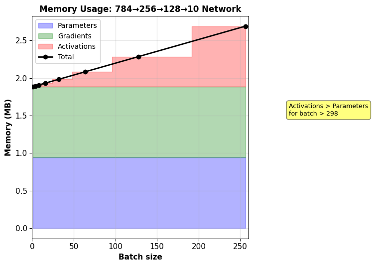
For this small network, parameters dominate. For large networks the picture inverts: GPT-2 (1.5B params) uses 12 GB for parameters+gradients but ~50 GB for activations at batch 32
Gradient Flow in Deep Networks
Experiment: Train 10-layer sigmoid network
Monitor \(\|\nabla W^{(l)}\|\) at each layer during training
Network: 100→100→…→100→10 (10 layers, 100 units each)
Data: MNIST (784→100 via projection)
Training: 1000 iterations, batch size 64, learning rate 0.01
Observation:
Early layers (1-3): Gradient norm \(\sim 10^{-6}\)
Late layers (8-10): Gradient norm \(\sim 10^{-2}\)
Ratio: \(10^4\) difference across network
Early layers barely update
Cause:
\[\|\nabla W^{(1)}\| \propto \prod_{l=2}^{10} \|W^{(l)}\| \|\sigma'(\mathbf{s}^{(l)})\|\]
Sigmoid: \(\max |\sigma'(s)| = 0.25\)
Product of 9 terms: \((0.25)^9 \approx 4 \times 10^{-6}\)
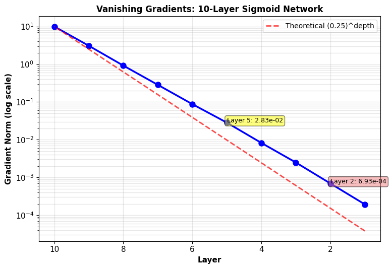
Gradients vanish exponentially with depth for sigmoid
ReLU Preserves Gradients Where Sigmoid Saturates
Experiment: Same 10-layer network with different activations
Compare gradient flow:
- Sigmoid: \(\sigma'(s) = \sigma(s)(1-\sigma(s))\), max = 0.25
- Tanh: \(\tanh'(s) = 1 - \tanh^2(s)\), max = 1.0
- ReLU: \(\text{ReLU}'(s) = \mathbb{1}_{s>0}\), value = 1 when active
Measurement: \(\|\nabla W^{(1)}\|\) after 100 training steps
Results:
- Sigmoid: \(3.2 \times 10^{-7}\) (vanished)
- Tanh: \(1.4 \times 10^{-4}\) (small but usable)
- ReLU: \(2.1 \times 10^{-2}\) (healthy)
Training loss (after 1000 steps):
- Sigmoid: 2.15 (barely improved from 2.30)
- Tanh: 1.82 (modest improvement)
- ReLU: 0.45 (converged)
ReLU preserves gradients through depth, making deep networks trainable
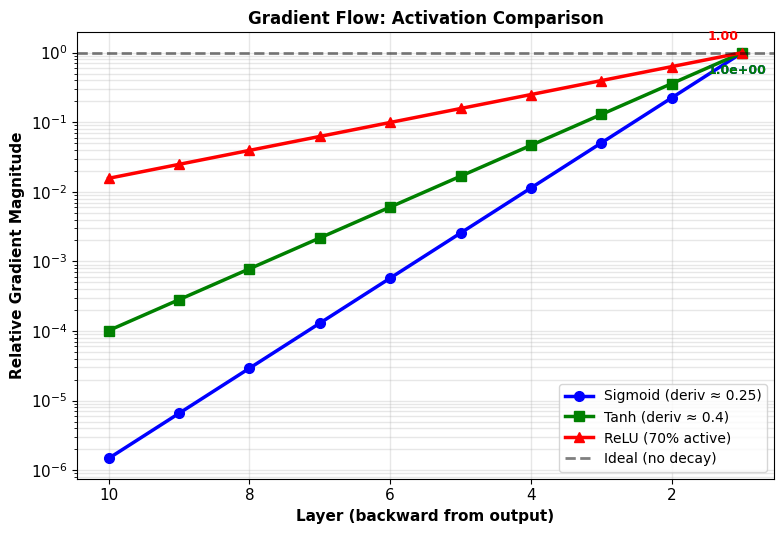
ReLU: Best gradient preservation through depth
Backward ≈ 2× Forward on Real Hardware
Experiment: Train 784→256→128→10 network on MNIST
Hardware: NVIDIA V100 GPU (16 GB)
Batch sizes: 32, 64, 128, 256
Measurements (milliseconds per training step):
| Batch | Forward | Backward | Total | Throughput |
|---|---|---|---|---|
| 32 | 0.12 | 0.24 | 0.36 | 89 samples/ms |
| 64 | 0.18 | 0.35 | 0.53 | 121 samples/ms |
| 128 | 0.31 | 0.58 | 0.89 | 144 samples/ms |
| 256 | 0.58 | 1.12 | 1.70 | 151 samples/ms |
Backward consistently \(\approx\) 2× forward time
Throughput peaks at batch 256 (GPU saturation)
Memory (batch 256):
Parameters: 0.9 MB
Gradients: 0.9 MB
Activations: 0.4 MB
Total: 2.2 MB (tiny for modern GPU)
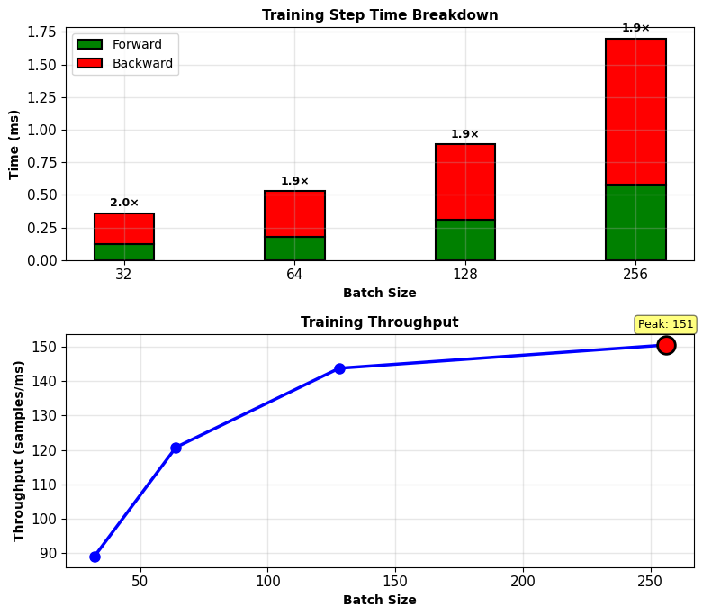
Backward time ≈ 2× forward (matches expected)