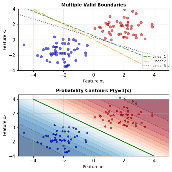
Classification – Mapping Features to Class Probabilities
Task: Given features \(\mathbf{x} \in \mathbb{R}^d\), predict class \(y \in \{0, 1\}\)
Classical approach: Find decision boundary
\[\hat{y} = \begin{cases}
1 & \text{if } f(\mathbf{x}) > 0 \\
0 & \text{otherwise}
\end{cases}\]
Probabilistic approach: Estimate \(P(y=1|\mathbf{x})\)
\[\hat{p} = P(y=1|\mathbf{x}) \in [0, 1]\]
\[\hat{y} = \mathbb{1}[\hat{p} > \tau]\]
Main challenges:
- How do we model \(P(y|\mathbf{x})\)?
- What loss function captures objective?
- What threshold \(\tau\) minimizes expected cost?
Threshold Rules Convert Probabilities to Labels
Classification pipeline:
- Model: Estimate \(P(y=1|\mathbf{x})\)
- Training: Learn parameters from data
- Inference: Compute \(p = P(y=1|\mathbf{x}_{\text{new}})\)
- Decision: Choose \(\hat{y} \in \{0, 1\}\)
The decision rule maps \(p\) to \(\hat{y}\):
Simple threshold:
\[\hat{y} = \begin{cases}
1 & p > 0.5 \\
0 & p \leq 0.5
\end{cases}\]
This assumes all errors cost the same
Example: Credit card fraud
- False positive: Block legitimate transaction ($10 cost)
- False negative: Approve fraud ($1000 loss)
Optimal threshold depends on these costs
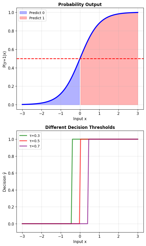
Different thresholds lead to different decisions
Decision Theory – States, Actions, Rules, and Loss
-
States (observations): \(\Omega = \{\omega_1, \omega_2, \ldots\}\)
- True class labels: \(y \in \{0, 1\}\) or \(\{1, 2, \ldots, K\}\)
-
Actions: \(\mathcal{A} = \{a_1, a_2, \ldots\}\)
- Predicted labels: \(\hat{y}\)
- Or “reject” option (defer to human)
-
Decision rule: \(\delta: \mathcal{X} \to \mathcal{A}\)
- Maps observations to actions
-
Loss function: \(L: \Omega \times \mathcal{A} \to \mathbb{R}\)
- Cost of action \(a\) when true state is \(\omega\)
Objective: Minimize expected loss
\[R(\delta) = \mathbb{E}[L(Y, \delta(X))]\]
Bayes risk: Minimum achievable expected loss
\[R^* = \inf_\delta R(\delta)\]
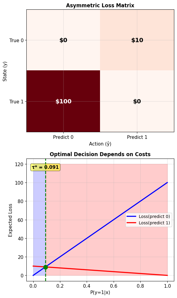
Bayesian Decision Theory Foundation
Bayes risk minimization:
Given observation \(\mathbf{x}\), choose action to minimize expected loss:
\[\delta^*(\mathbf{x}) = \arg\min_{a \in \mathcal{A}} \mathbb{E}[L(Y, a) | \mathbf{X} = \mathbf{x}]\]
Expanding the expectation:
\[= \arg\min_{a} \sum_{k} L(k, a) \cdot P(Y=k|\mathbf{x})\]
For binary classification with \(y \in \{0, 1\}\):
\[\delta^*(\mathbf{x}) = \arg\min_{a \in \{0,1\}} \left[ L(0,a)(1-p) + L(1,a)p \right]\]
where \(p = P(Y=1|\mathbf{x})\)
Optimal decisions depend on:
- Posterior probabilities \(P(Y=k|\mathbf{x})\)
- Loss function \(L(k, a)\)
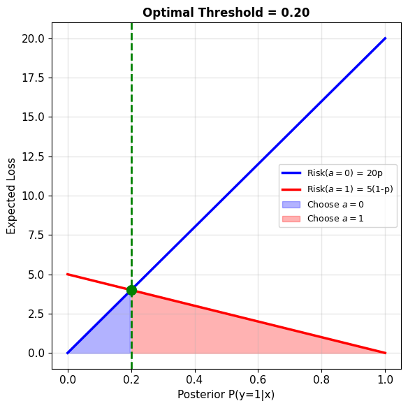
Bayes rule minimizes expected loss at each point
Uniform Loss Leads to MAP Rule
0-1 Loss (uniform error cost):
\[L(y, \hat{y}) = \begin{cases}
0 & \text{if } y = \hat{y} \\
1 & \text{if } y \neq \hat{y}
\end{cases}\]
Expected loss for action \(a\):
\[\mathbb{E}[L(Y, a) | \mathbf{x}] = \sum_{k \neq a} P(Y=k|\mathbf{x}) = 1 - P(Y=a|\mathbf{x})\]
Minimizing expected loss:
\[\delta^*(\mathbf{x}) = \arg\min_a [1 - P(Y=a|\mathbf{x})] = \arg\max_a P(Y=a|\mathbf{x})\]
This is the MAP rule!
\[\boxed{\delta_{\text{MAP}}(\mathbf{x}) = \arg\max_k P(Y=k|\mathbf{x})}\]
MAP minimizes error probability when all errors cost the same
Bayes error rate (irreducible error):
\[\epsilon^* = \mathbb{E}[1 - \max_k P(Y=k|X)]\]
No classifier can do better — this is the error from class overlap
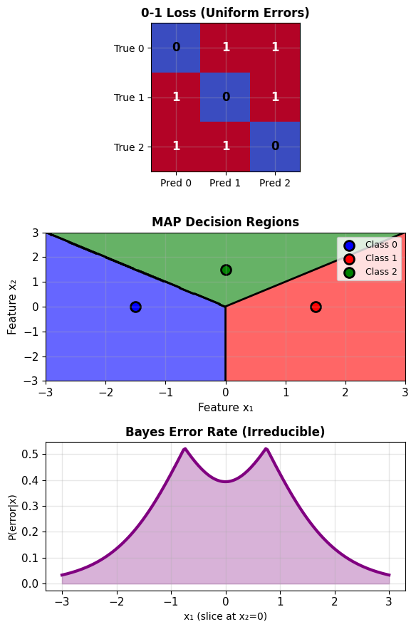
Each region: highest posterior probability wins
Likelihood Ratio Test for Binary Classification
Binary Bayes decision rule:
Choose class 1 if “expected loss of choosing 1” < “expected loss of choosing 0”:
\[L_{01}P(Y=0|\mathbf{x}) < L_{10}P(Y=1|\mathbf{x})\]
where \(L_{ij}\) = loss of predicting \(j\) when true class is \(i\)
Using Bayes theorem:
\[P(Y=k|\mathbf{x}) = \frac{p(\mathbf{x}|Y=k)P(Y=k)}{p(\mathbf{x})}\]
Rearranging:
\[\frac{p(\mathbf{x}|Y=1)}{p(\mathbf{x}|Y=0)} > \frac{L_{01}P(Y=0)}{L_{10}P(Y=1)}\]
Likelihood Ratio Test:
\[\boxed{\Lambda(\mathbf{x}) = \frac{p(\mathbf{x}|Y=1)}{p(\mathbf{x}|Y=0)} \underset{H_0}{\overset{H_1}{\gtrless}} \tau}\]
where threshold \(\tau = \frac{L_{01}P(Y=0)}{L_{10}P(Y=1)}\)
Log-likelihood ratio (more stable):
\[\log \Lambda(\mathbf{x}) = \log p(\mathbf{x}|Y=1) - \log p(\mathbf{x}|Y=0)\]
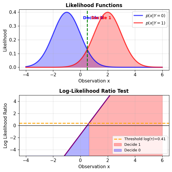
Linear boundary in log-space → stability
When Errors Have Different Costs
Binary classification with costs:
\[L = \begin{bmatrix}
0 & c_{01} \\
c_{10} & 0
\end{bmatrix}\]
where:
- \(c_{01}\): Cost of false positive (say 1 when true is 0)
- \(c_{10}\): Cost of false negative (say 0 when true is 1)
Expected loss of predicting 1:
\[R_1(\mathbf{x}) = c_{01} \cdot P(y=0|\mathbf{x})\]
Expected loss of predicting 0:
\[R_0(\mathbf{x}) = c_{10} \cdot P(y=1|\mathbf{x})\]
Optimal decision: Predict 1 if \(R_1(\mathbf{x}) < R_0(\mathbf{x})\)
\[c_{01}(1-p) < c_{10} \cdot p\]
\[p > \frac{c_{01}}{c_{01} + c_{10}}\]
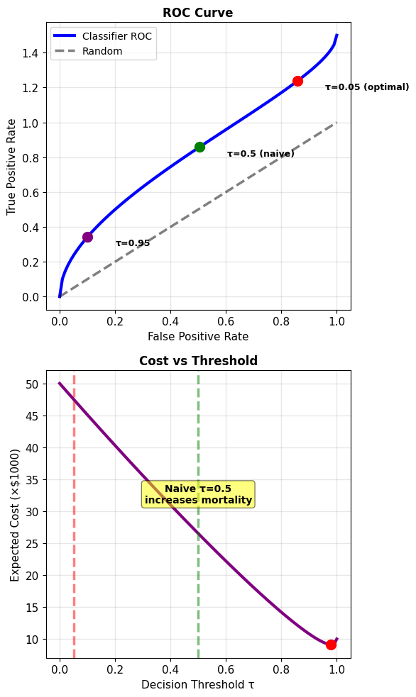
Optimal threshold: \(\tau^* = \frac{c_{01}}{c_{01} + c_{10}}\)
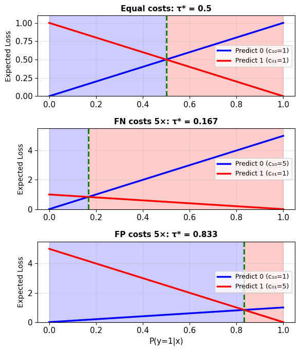
Medical Diagnosis as a Decision Problem
Cancer screening scenario:
- State: Cancer (1) or Healthy (0)
- Action: Treat (1) or Don’t treat (0)
Realistic costs:
- False negative (miss cancer): Death = $1,000,000
- False positive (unnecessary treatment): $50,000
- True positive (treat cancer): $50,000
- True negative (no treatment): $0
Loss matrix:
\[L = \begin{bmatrix}
0 & 50,000 \\
1,000,000 & 50,000
\end{bmatrix}\]
Note: treatment cost even for true positives
Optimal threshold:
\[\tau^* = \frac{50,000}{50,000 + 950,000} = 0.05\]
Treat if \(P(\text{cancer}|\text{test}) > 0.05\)
Rejecting – Deferring When Confidence Is Low
Three-way decision:
- Predict class 0
- Predict class 1
- Reject (defer to expert)
Extended loss matrix:
\[L = \begin{bmatrix}
0 & c_{01} & c_r \\
c_{10} & 0 & c_r
\end{bmatrix}\]
where \(c_r\) = cost of rejection (expert review)
Decision regions:
- Predict 0 if \(p < \tau_1\)
- Reject if \(\tau_1 \leq p \leq \tau_2\)
- Predict 1 if \(p > \tau_2\)
Optimal thresholds (for symmetric costs):
\[\tau_1 = \frac{c_r}{c_{10}}, \quad \tau_2 = 1 - \frac{c_r}{c_{01}}\]
Reject when model confidence is low
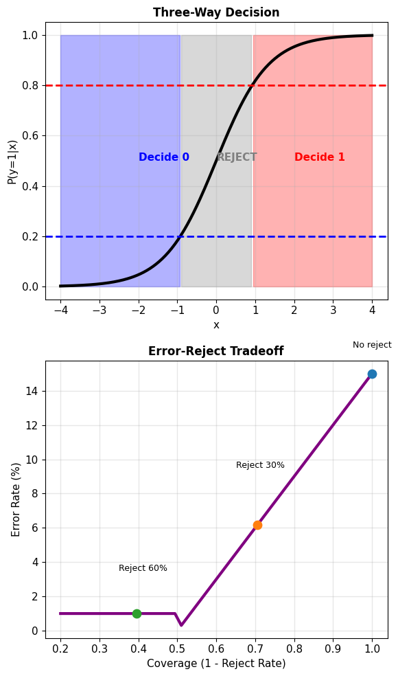
Reject option reduces error on uncertain samples
Extending Bayes Decisions to K Classes
:::: {.columns}
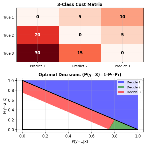
K-class cost matrix: \(L \in \mathbb{R}^{K \times K}\)
\[L_{ij} = \text{cost of predicting } j \text{ when true is } i\]
Expected loss for action \(a\):
\[R_a(\mathbf{x}) = \sum_{k=1}^K L_{ka} \cdot P(y=k|\mathbf{x})\]
Optimal decision:
\[\hat{y}^* = \arg\min_a R_a(\mathbf{x})\]
Example: 3-class with varying costs
\[L = \begin{bmatrix}
0 & 5 & 10 \\
20 & 0 & 5 \\
30 & 15 & 0
\end{bmatrix}\]
Must compute expected loss for each action
Special case: If \(L_{ij} = 1 - \delta_{ij}\) (0-1 loss), reduces to argmax of posteriors
:::
Soft Decisions Preserve Uncertainty for Downstream Use
Hard decisions: \(\hat{y} \in \{0, 1, ..., K-1\}\)
- Single class prediction
- Required for final action
- Information loss through discretization
Soft decisions: \(\mathbf{p} = [p_0, p_1, ..., p_{K-1}]\)
- Full distribution of outcomes
- Preserves uncertainty information
- Useful for downstream processing
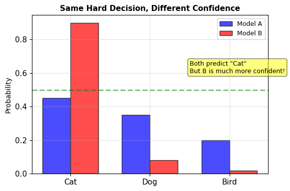
Soft decisions ideal for:
-
Cascaded systems: Next stage uses probabilities
- Speech recognition → language model
- Object detection → tracking
-
Confidence assessment: Reliability measures
- Medical diagnosis (refer if uncertain)
- Autonomous driving (hand off to human)
-
Cost-sensitive decisions: Context-dependent losses
- Fraud detection (amount matters)
- Email filtering (sender importance)
-
Ensemble methods: Combining multiple models
Beyond Accuracy – Evaluating Probabilistic Classifiers
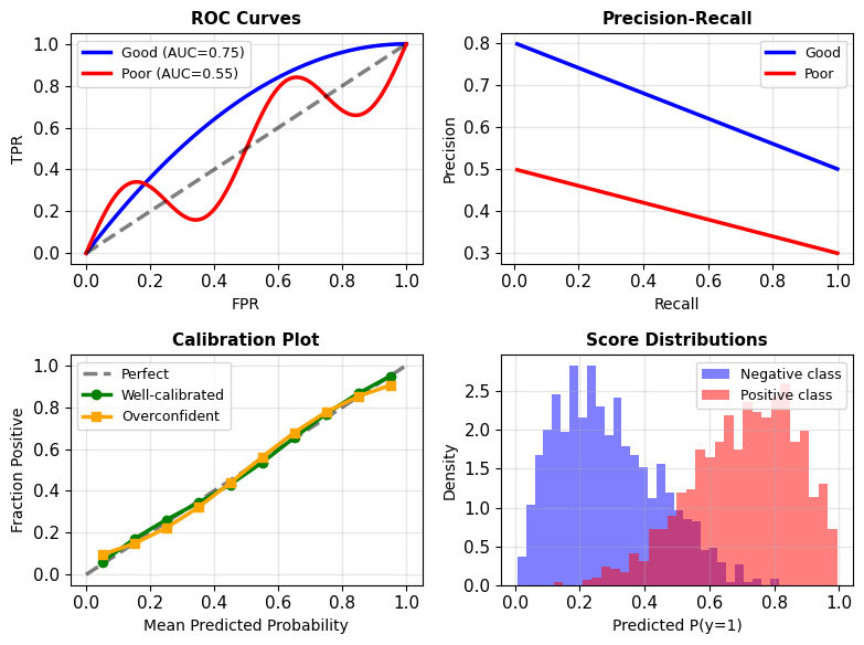
1. Discrimination (ranking ability):
- ROC curve: TPR vs FPR
- AUC: Area under ROC
- Precision-Recall curve
2. Calibration (probability accuracy):
- Do predicted probabilities match frequencies?
- Among all \(\mathbf{x}\) where \(P(y=1|\mathbf{x}) = 0.7\), is the true fraction positive ≈ 70%?
3. Proper scoring rules:
- Log-loss: \(-\sum_i [y_i \log p_i + (1-y_i)\log(1-p_i)]\)
- Brier score: \(\sum_i (y_i - p_i)^2\)
These penalize both discrimination and calibration errors
Note: Good discrimination ≠ Good calibration
Class Imbalance Makes Accuracy Misleading
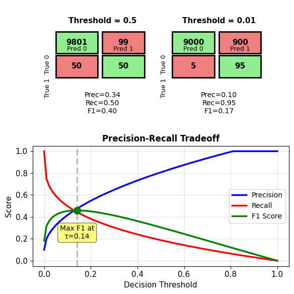
Imbalanced data: 99% negative, 1% positive
Problem with accuracy:
- Trivial classifier (always predict negative): 99% accurate
- Does not detect rare positive cases
Metrics for imbalanced data:
Precision: Of predicted positives, how many correct?
\[\text{Precision} = \frac{\text{TP}}{\text{TP} + \text{FP}}\]
Recall (Sensitivity): Of true positives, how many found?
\[\text{Recall} = \frac{\text{TP}}{\text{TP} + \text{FN}}\]
F1 Score: Harmonic mean
\[F_1 = \frac{2 \cdot \text{Precision} \cdot \text{Recall}}{\text{Precision} + \text{Recall}}\]
Connection to costs: Optimize threshold based on
\[\tau^* = \frac{c_{01} \cdot (1-\pi)}{c_{01}(1-\pi) + c_{10} \cdot \pi}\]
where \(\pi\) = class prior P(y=1)
Why Linear Models Fail
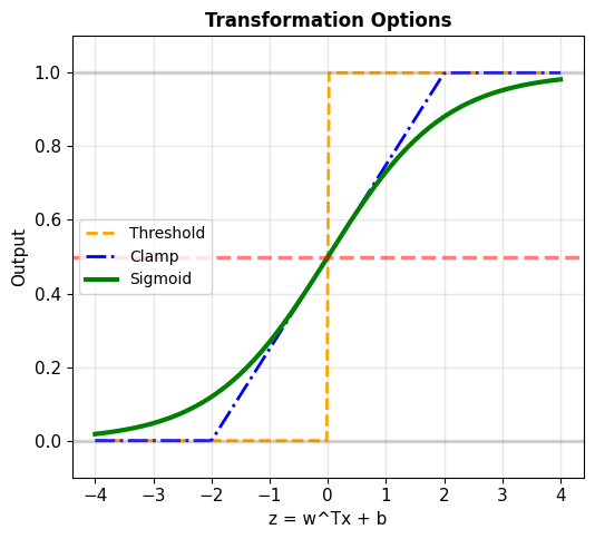
Try modeling probability directly:
\[p(\mathbf{x}) = \mathbf{w}^T\mathbf{x} + b\]
With \(w = 0.3\), \(b = 0.5\):
- \(p(x=-2) = -0.1\) (invalid)
- \(p(x=0) = 0.5\)
- \(p(x=2) = 1.1\) (invalid)
Problem: Linear outputs \(\in (-\infty, \infty)\) but probabilities need \(\in [0, 1]\)
Need transformation \(\mathbb{R} \to [0, 1]\) that:
- Outputs valid probabilities
- Preserves linear decision boundaries
- Is differentiable for optimization
Candidates:
- Threshold: \(p = \mathbb{1}[z > 0]\)
- Clamp: \(p = \max(0, \min(1, z))\) – Not differentiable
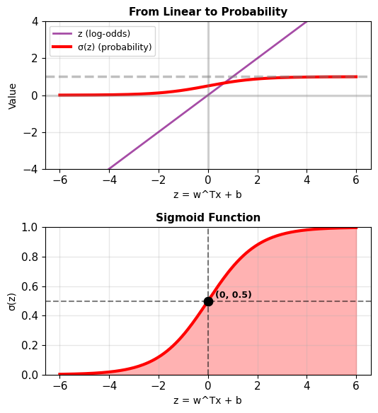
- Sigmoid: \(p = \frac{1}{1 + e^{-z}}\)
Log-Odds Map Probabilities to the Real Line
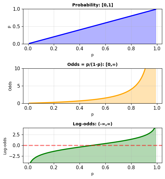
Odds: Alternative to probability
\[\text{Odds}(A) = \frac{P(A)}{P(A^C)}\]
For binary outcome
\[\text{Odds} = \frac{p}{1-p} = \frac{P(y=1)}{P(y=0)}\]
Examples:
- \(p = 0.5\): Odds = 1 (1:1, “even odds”)
- \(p = 0.75\): Odds = 3 (3:1 in favor)
- \(p = 0.25\): Odds = 1/3 (1:3 against)
Range: \([0, \infty)\)
Log-odds (logit):
\[\text{logit}(p) = \log\left(\frac{p}{1-p}\right)\]
Range: \((-\infty, \infty)\)
The Logistic Model
Model log-odds linearly:
\[\log\left(\frac{p(\mathbf{x})}{1-p(\mathbf{x})}\right) = \mathbf{w}^T\mathbf{x} + b\]
Solving for \(p(\mathbf{x})\):
Let \(z = \mathbf{w}^T\mathbf{x} + b\)
\[\frac{p}{1-p} = e^z\]
\[p = (1-p)e^z\]
\[p = e^z - pe^z\]
\[p(1 + e^z) = e^z\]
\[p = \frac{e^z}{1 + e^z} = \frac{1}{1 + e^{-z}}\]
Gives the logistic (sigmoid) function
\[\boxed{p(\mathbf{x}) = \sigma(\mathbf{w}^T\mathbf{x} + b) = \frac{1}{1 + e^{-(\mathbf{w}^T\mathbf{x} + b)}}}\]
The Sigmoid Unit
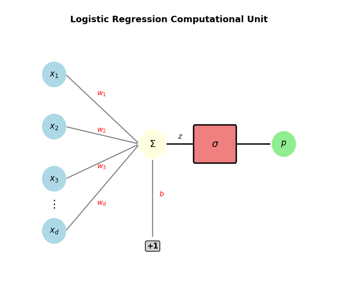
Inputs: \(\mathbf{x} = [x_1, x_2, \ldots, x_d]^T\)
Weights: \(\mathbf{w} = [w_1, w_2, \ldots, w_d]^T\)
Bias: \(b\)
Linear combination:
\[z = \mathbf{w}^T\mathbf{x} + b = \sum_{j=1}^d w_j x_j + b\]
Activation function:
\[p = \sigma(z) = \frac{1}{1 + e^{-z}}\]
Output: \(p = P[\text{class 1}] \in (0, 1)\)
Decision rule: Predict class 1 if \(p > 0.5\)
Why Log-Odds (Not Other Transformations)?
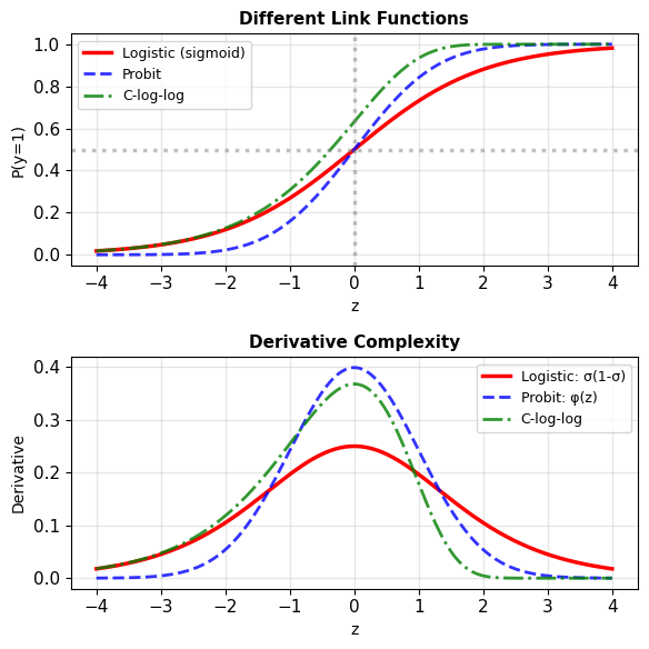
Other candidates that map \(\mathbb{R} \to [0,1]\):
Probit (cumulative normal):
\[p = \Phi(z) = \int_{-\infty}^z \frac{1}{\sqrt{2\pi}}e^{-t^2/2}dt\]
- No closed form
- Derivative involves normal PDF
- Used in econometrics
Complementary log-log:
\[p = 1 - e^{-e^z}\]
- Asymmetric
- Good for rare events
- Different tail behavior
Logistic function advantages:
- Natural interpretation: Log-odds are intuitive
- Simple derivative: \(\sigma'(z) = \sigma(z)(1-\sigma(z))\)
- Computational efficiency: Closed form everything
- Information theory: Maximizes entropy given constraints
Sigmoid – Valid Probabilities, Linear Boundaries, Interpretable Weights
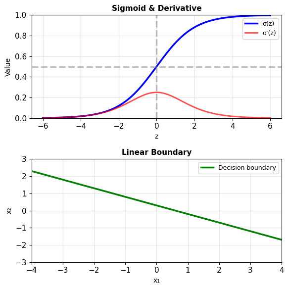
The sigmoid function \(\sigma(z) = \frac{1}{1 + e^{-z}}\):
-
Valid probabilities: \(\sigma(z) \in (0, 1)\) always
-
Smooth and differentiable:
\[\sigma'(z) = \sigma(z)(1 - \sigma(z))\] -
Linear decision boundary:
- Predict 1 if \(p > 0.5\)
- This occurs when \(\mathbf{w}^T\mathbf{x} + b > 0\)
- Boundary: \(\mathbf{w}^T\mathbf{x} + b = 0\) (hyperplane)
-
Interpretable coefficients:
- \(w_j\) = change in log-odds per unit \(x_j\)
- \(e^{w_j}\) = odds multiplication factor
When the Log-Odds Linearity Assumption Breaks
Logistic regression assumes:
\[\log\frac{P(y=1|\mathbf{x})}{P(y=0|\mathbf{x})} = \mathbf{w}^T\mathbf{x} + b\]
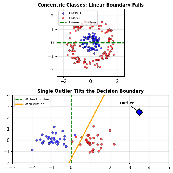
Nonlinear boundaries: Concentric classes, XOR — no linear \(f(\mathbf{x})\) works
- Best linear classifier on XOR: 50% accuracy
- More data doesn’t help — the model class is wrong
Outlier sensitivity: One extreme point pulls \(\|\mathbf{w}\| \to \infty\)
- MLE maximizes confidence on every sample
- No mechanism to downweight outliers
High dimensions (\(d > n\)): Perfect separation \(\Rightarrow\) \(\hat{\mathbf{w}}_{\text{MLE}}\) diverges
- 100 features, 80 samples: \(\|\mathbf{w}\|\) grows without bound
- Regularization (Section 5) fixes this
Misspecification: MLE finds best sigmoid approximation in KL divergence
\[\hat{\mathbf{w}} = \arg\min_{\mathbf{w}} D_{\text{KL}}(p_{\text{true}} \| p_{\sigma}(\cdot; \mathbf{w}))\]
Finding \(\mathbf{w}\) and \(b\) That Fit the Data
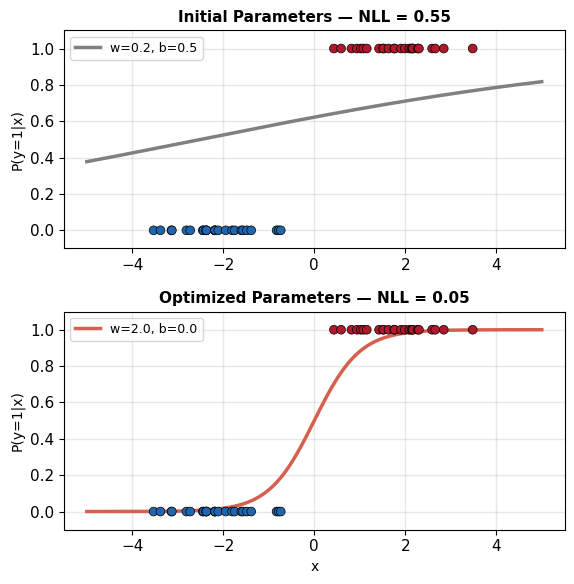
Model: \(P(y=1|\mathbf{x}) = \sigma(\mathbf{w}^T\mathbf{x} + b)\)
Training data: \(\{(\mathbf{x}_i, y_i)\}_{i=1}^n\)
Objective: Find \(\mathbf{w}, b\) that make observed labels most probable
\[\hat{\mathbf{w}} = \arg\max_{\mathbf{w}} \prod_{i=1}^n p_i^{y_i}(1-p_i)^{1-y_i}\]
Equivalent to minimizing cross-entropy:
\[\mathcal{L} = -\sum_{i=1}^n [y_i \log p_i + (1-y_i)\log(1-p_i)]\]
Gradient: \(\nabla_\mathbf{w} \ell = \sum_{i=1}^n (y_i - p_i)\mathbf{x}_i\)
Errors weighted by features — intuitive and cheap to compute
Example: Spam Detection
Problem: Classify emails as spam or legitimate
Features extracted from email:
- Word frequencies: “FREE”, “CLICK”, “offer”
- Sender reputation score
- Number of ALL CAPS words
- Exclamation marks count
- Links to external domains
- Time of day sent
Example vector \(\mathbf{x} \in \mathbb{R}^6\):
Email: "FREE OFFER! Click HERE!!!"
x = [2, 0.1, 2, 3, 1, 0.3]
     ↑   ↑   ↑   ↑   ↑   ↑
   FREE low  2   3   1   3am
   offer rep CAPS !!  link
In practice, \(d\) = 100–10,000 features (bag-of-words counts, TF-IDF weights, metadata)
Goal: Learn \(P(\text{spam}|\mathbf{x})\)
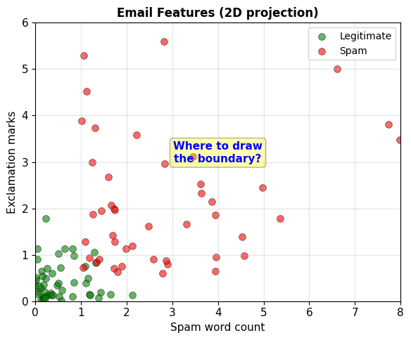
Spam filters use 1000s of features
Training Logistic Regression
Model:
\[P(\text{spam}|\mathbf{x}) = \sigma(\mathbf{w}^T\mathbf{x} + b)\]
Training (gradient ascent on log-likelihood):
# Initialize
w = np.random.randn(100) * 0.01
b = 0

for epoch in range(100):
    # Compute predictions
    z = X @ w + b
    p = sigmoid(z)

    # Gradient step
    grad_w = X.T @ (y - p) / n
    grad_b = np.mean(y - p)

    w += learning_rate * grad_w
    b += learning_rate * grad_b
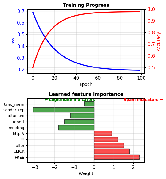
Learned weights reveal spam indicators:
- \(w_{\text{FREE}} = 2.3\) (strong spam signal)
- \(w_{\text{meeting}} = -1.8\) (legitimate signal)
- \(w_{\text{sender_rep}} = -3.1\) (reputation matters)
Target: >95% detection, <0.1% false positive, <10ms latency
Calibrated Probabilities Enable Threshold Tuning
Inference for new email:
def classify_email(email_text, w, b):
    # Extract features
    x = extract_features(email_text)

    # Compute probability
    z = np.dot(w, x) + b
    p_spam = sigmoid(z)

    # Decision with threshold
    if p_spam > 0.95:  # High threshold
        return "spam", p_spam
    else:
        return "legitimate", p_spam
Example performance:
- Accuracy: 97.2%
- Spam recall: 95.1%
- False positive rate: 0.08%
- Inference time: 0.3ms per email
Advantages:
- Interpretable: see why email flagged
- Fast: millions of emails per second
- Updatable: online learning for new spam
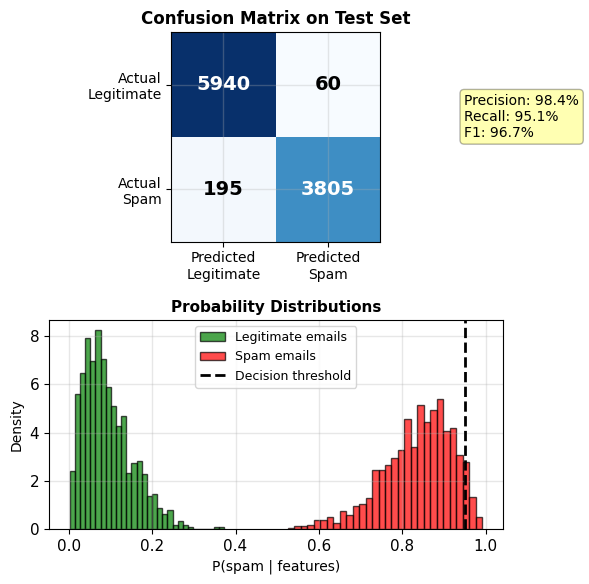
Threshold tuning possible since calibrated probabilities
Example: MLE with 4 Points – Compute the Likelihood
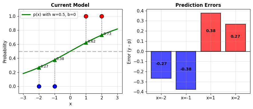
Dataset: 4 points in 1D
X = [-2, -1, 1, 2]
y = [0, 0, 1, 1]
Current Model: \(p(x) = \sigma(wx + b)\)
with \(w = 0.5\), \(b = 0\)
Compute predictions:
- \(z_1 = 0.5(-2) + 0 = -1\), \(p_1 = \sigma(-1) = 0.27\)
- \(z_2 = 0.5(-1) + 0 = -0.5\), \(p_2 = \sigma(-0.5) = 0.38\)
- \(z_3 = 0.5(1) + 0 = 0.5\), \(p_3 = \sigma(0.5) = 0.62\)
- \(z_4 = 0.5(2) + 0 = 1\), \(p_4 = \sigma(1) = 0.73\)
Errors \(y - p\):
- Point 1: \(0 - 0.27 = -0.27\)
- Point 2: \(0 - 0.38 = -0.38\)
- Point 3: \(1 - 0.62 = +0.38\)
- Point 4: \(1 - 0.73 = +0.27\)
Log-Likelihood for the 4-Point Example
Log-likelihood:
\[\ell = \sum_{i=1}^4 [y_i \log p_i + (1-y_i)\log(1-p_i)]\]
So:
- \(i=1\): \(0 \cdot \log(0.27) + 1 \cdot \log(0.73) = -0.31\)
- \(i=2\): \(0 \cdot \log(0.38) + 1 \cdot \log(0.62) = -0.48\)
- \(i=3\): \(1 \cdot \log(0.62) + 0 \cdot \log(0.38) = -0.48\)
- \(i=4\): \(1 \cdot \log(0.73) + 0 \cdot \log(0.27) = -0.31\)
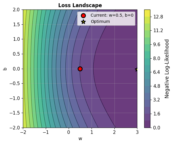
Total: \(\ell = -1.58\)
Negative log-likelihood: \(\text{NLL} = 1.58\)
Minimize this loss function
Gradient – Errors Weighted by Features
Gradient formulas (from earlier):
\[\frac{\partial \ell}{\partial w} = \sum_{i=1}^n (y_i - p_i)x_i\]
\[\frac{\partial \ell}{\partial b} = \sum_{i=1}^n (y_i - p_i)\]
For our example:
\(\frac{\partial \ell}{\partial w}\):
\[\begin{align}
&= (-0.27)(-2) + (-0.38)(-1)\\
&\quad + (0.38)(1) + (0.27)(2)\\
&= 0.54 + 0.38 + 0.38 + 0.54\\
&= 1.84
\end{align}\]
\(\frac{\partial \ell}{\partial b}\):
\[= -0.27 - 0.38 + 0.38 + 0.27 = 0\]
Computing contributions:
| \(i\) | \(x_i\) | \(y_i\) | \(p_i\) | \((y_i - p_i)x_i\) |
|---|---|---|---|---|
| 1 | -2 | 0 | 0.27 | 0.54 |
| 2 | -1 | 0 | 0.38 | 0.38 |
| 3 | 1 | 1 | 0.62 | 0.38 |
| 4 | 2 | 1 | 0.73 | 0.54 |
Sum: \(\nabla_w \ell = 1.84\)
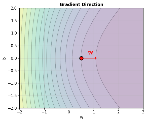
Gradient w.r.t. \(w\) positive: increase \(w\)
Gradient w.r.t. \(b\) zero: \(b\) locally optimal
Larger errors \(|y_i - p_i|\) contribute more to gradient.
The Complete Logistic Regression Training Loop
-
Model: \(p = \sigma(\mathbf{w}^T\mathbf{x} + b)\)
-
Objective: Maximize log-likelihood
\[\ell = \sum_{i=1}^n [y_i \log p_i + (1-y_i)\log(1-p_i)]\] -
Gradient:
\[\nabla_\mathbf{w} \ell = \mathbf{X}^T(\mathbf{y} - \mathbf{p})\] -
Update: Gradient ascent
\[\mathbf{w} \leftarrow \mathbf{w} + \eta \nabla_\mathbf{w} \ell\] -
Converge: When \(||\nabla \ell|| < \epsilon\)
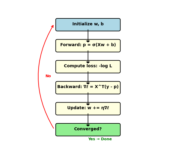
Iterate until convergence (typical: 100s of steps)
Initialize Weights Before Optimization
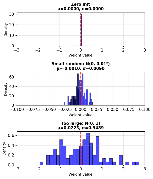
Standard initialization:
w = np.random.randn(d) * 0.01
b = 0
Why random: Zero works but random is standard
- Gradient: \(\nabla_\mathbf{w} \ell = \mathbf{X}^T(\mathbf{y} - \mathbf{p})\)
- Gradient depends only on data, not symmetry
- With \(\mathbf{w} = \mathbf{0}\): all predictions \(p_i = 0.5\)
- Works for logistic regression (unlike neural networks)
- Random initialization is standard practice
Why small (0.01 scale):
- Prevents sigmoid saturation: \(\sigma(z) \approx 0\) or \(1\) when \(|z|\) large
- Keeps gradients large: \(\sigma'(z) = \sigma(z)(1-\sigma(z))\) peaks at \(z=0\)
- Scale of 0.01 typical for normalized features
Gradient Descent — \(\nabla_\mathbf{w}\)
Update rule (minimize NLL):
\[\mathbf{w}^{\text{new}} = \mathbf{w}^{\text{old}} + \eta \cdot \nabla \ell\]
Addition follows from maximizing log-likelihood (equivalent to subtracting gradient of NLL)
With learning rate \(\eta = 0.5\):
- \(w^{\text{new}} = 0.5 + 0.5 \cdot 1.84 = 1.42\)
- \(b^{\text{new}} = 0 + 0.5 \cdot 0 = 0\)
New predictions:
- \(p_1^{\text{new}} = \sigma(1.42 \cdot (-2)) = 0.055\)
- \(p_2^{\text{new}} = \sigma(1.42 \cdot (-1)) = 0.195\)
- \(p_3^{\text{new}} = \sigma(1.42 \cdot 1) = 0.805\)
- \(p_4^{\text{new}} = \sigma(1.42 \cdot 2) = 0.945\)
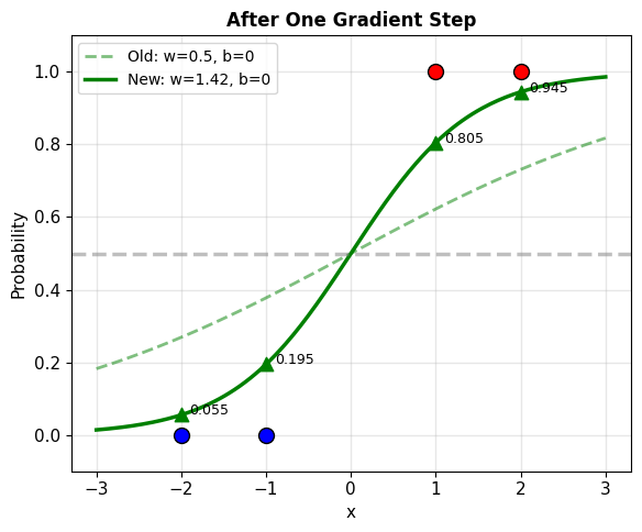
NLL decreased from 1.582 to 0.506
- Class 0 predictions closer to 0
- Class 1 predictions closer to 1
- Better separation between classes
Convergence Analysis (Gradient Descent)
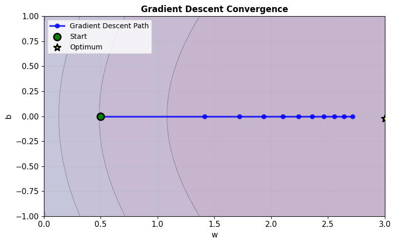
Convexity guarantees convergence to global optimum
Why Is Logistic Regression Convex?
Theorem: NLL is strictly convex if \(\mathbf{X}\) has full rank.
Proof sketch:
-
Hessian: \(\mathbf{H} = -\mathbf{X}^T\mathbf{D}\mathbf{X}\)
-
For any \(\mathbf{v} \neq \mathbf{0}\):
\[\mathbf{v}^T(-\mathbf{H})\mathbf{v} = \mathbf{v}^T\mathbf{X}^T\mathbf{D}\mathbf{X}\mathbf{v}\] -
Let \(\mathbf{u} = \mathbf{X}\mathbf{v}\):
\[= \mathbf{u}^T\mathbf{D}\mathbf{u} = \sum_{i=1}^n p_i(1-p_i)u_i^2\] -
Since \(0 < p_i < 1\): all \(p_i(1-p_i) > 0\)
-
Sum of positive terms → \(\geq 0\)
-
Equals 0 only if \(\mathbf{u} = \mathbf{0}\)
-
If \(\mathbf{X}\) full rank: \(\mathbf{X}\mathbf{v} = \mathbf{0} \Rightarrow \mathbf{v} = \mathbf{0}\)
-
Therefore: \(-\mathbf{H} \succ 0\) (positive definite)
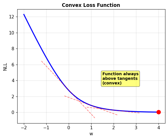
Convexity implications:
| Property | Convex (Logistic) | Non-convex (Neural Net) |
|---|---|---|
| Local minima | None (only global) | Many |
| Optimization | Any method works | Can get stuck |
| Convergence | Guaranteed | No guarantee |
| Initial point | Doesn’t matter | Critical |
| Solution | Unique (if full rank) | Multiple |
Newton’s Method Converges Quadratically
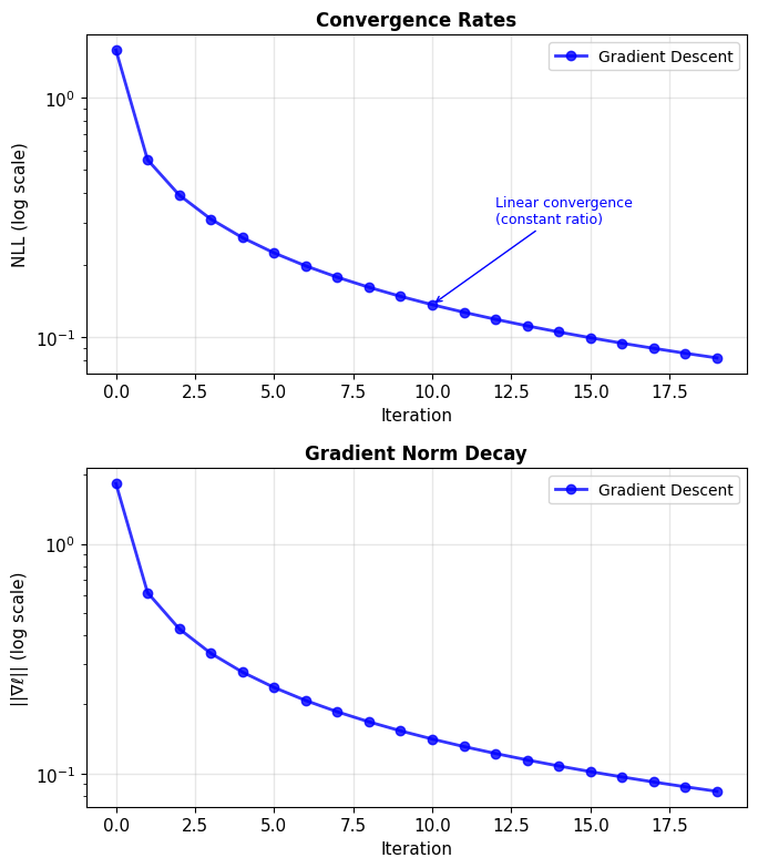
Gradient Descent:
- Linear convergence: \(\epsilon_{t+1} \leq \rho \cdot \epsilon_t\)
- Rate depends on condition number
- Many iterations needed
- Simple, memory efficient
Newton’s Method:
- Quadratic convergence: \(\epsilon_{t+1} \leq c \cdot \epsilon_t^2\)
- Few iterations (5-10 typical)
- Each iteration expensive: \(O(d^3)\)
- Needs to store/invert Hessian
Trade-off:
- Small \(d\) (<1000): Use Newton
- Large \(d\): Use gradient methods
- Very large \(d\): Use stochastic gradient
Fisher Information Measures Parameter Certainty
Fisher Information measures parameter certainty:
\[\mathcal{I} = \mathbb{E}[-\mathbf{H}] = \mathbb{E}[\mathbf{X}^T\mathbf{D}\mathbf{X}]\]
At convergence for our example:
- \(w^* \approx 2.2\), \(b^* \approx 0\)
- \(p^* = [0.013, 0.050, 0.950, 0.987]\)
Weights at optimum:
- Points 1,4: \(p(1-p) \approx 0.013\) (low)
- Points 2,3: \(p(1-p) \approx 0.048\) (low)
Low weights everywhere → High certainty
Asymptotic distribution:
\[\hat{\mathbf{w}} \sim \mathcal{N}(\mathbf{w}^*, \mathcal{I}^{-1}/n)\]
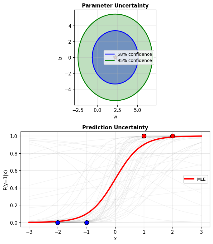
High Fisher information → Low variance → Confident estimates
From Binary to K > 2 Classes
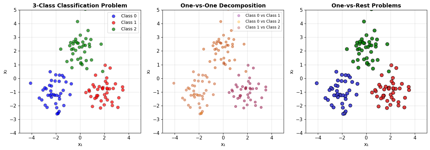
Why One-vs-Rest Fails
One-vs-Rest approach:
- Train K binary classifiers
- Classifier k: class k vs all others
- Predict: argmax of K outputs
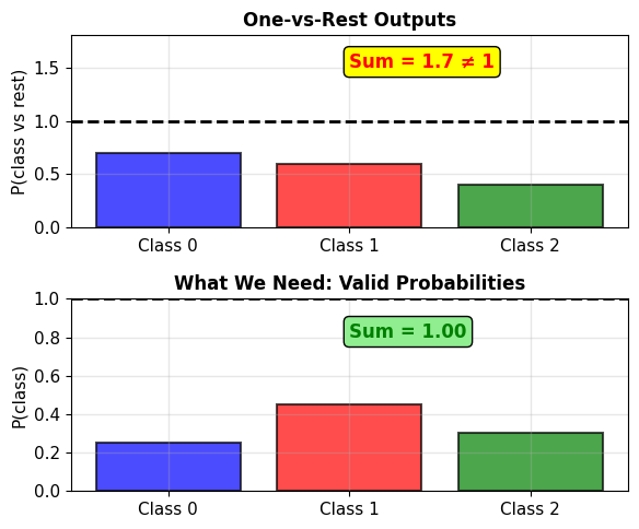
Problem: Probabilities do not sum to 1
Example with 3 classes:
- Classifier 0: P(0 vs rest) = 0.7
- Classifier 1: P(1 vs rest) = 0.6
- Classifier 2: P(2 vs rest) = 0.4
Sum = 1.7 ≠ 1
Not valid probabilities for the K classes
The Softmax Function
Generalize sigmoid to K dimensions:
\[\text{softmax}(\mathbf{z})_k = \frac{e^{z_k}}{\sum_{j=1}^K e^{z_j}}\]
For binary case (K=2):
- Let \(z_1 = 0\) (reference class)
- Then: \(p_2 = \frac{e^{z_2}}{e^0 + e^{z_2}} = \frac{1}{1 + e^{-z_2}} = \sigma(z_2)\)
Softmax reduces to sigmoid when K=2
Softmax Guarantees Valid Probability Distributions
-
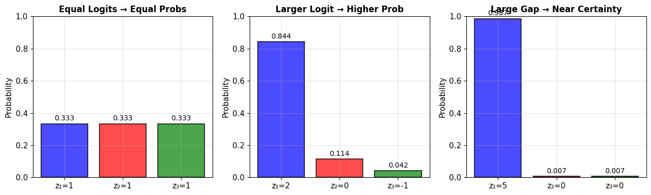
Valid probabilities: All outputs in (0,1), sum to 1
\[\sum_{k=1}^K \text{softmax}(\mathbf{z})_k = 1\] -
Preserves order: If \(z_i > z_j\), then \(p_i > p_j\)
-
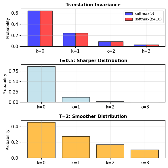
Translation invariant:
\[\text{softmax}(\mathbf{z} + c) = \text{softmax}(\mathbf{z})\]Since: \(\frac{e^{z_k + c}}{\sum_j e^{z_j + c}} = \frac{e^c \cdot e^{z_k}}{e^c \cdot \sum_j e^{z_j}} = \frac{e^{z_k}}{\sum_j e^{z_j}}\)
-
Temperature scaling:
\[\text{softmax}(\mathbf{z}/T)\]- \(T \to 0\): approaches argmax (one-hot)
- \(T \to \infty\): uniform distribution
Numerical Stability of Softmax
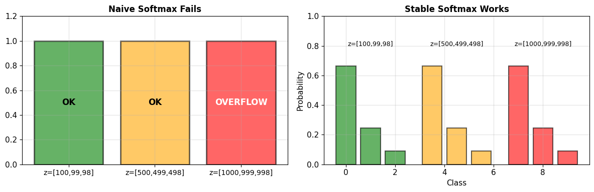
Problem: Exponentials overflow/underflow
z = [1000, 999, 998]
exp(1000) → inf  # Overflow
Solution: Take advantage of translation invariance
Subtract maximum before exponent
\[\text{softmax}(\mathbf{z}) = \text{softmax}(\mathbf{z} - \max(\mathbf{z}))\]
z = [1000, 999, 998]
z_stable = z - max(z) = [0, -1, -2]
softmax(z_stable) = [0.665, 0.245, 0.090]  # Valid
Multinomial Logistic Regression – One Linear Model per Class
For K classes, we need:
- K linear models: \(z_k = \mathbf{w}_k^T\mathbf{x} + b_k\)
- Parameter matrix: \(\mathbf{W} \in \mathbb{R}^{d \times K}\)
- Bias vector: \(\mathbf{b} \in \mathbb{R}^K\)
Model:
\[\mathbf{z} = \mathbf{W}^T\mathbf{x} + \mathbf{b}\]
\[P(y=k|\mathbf{x}) = \text{softmax}(\mathbf{z})_k\]
Over-parameterized:
- Can set \(\mathbf{w}_K = \mathbf{0}\), \(b_K = 0\) (reference class)
- Still get valid probabilities
- Reduces parameters by \(d+1\)
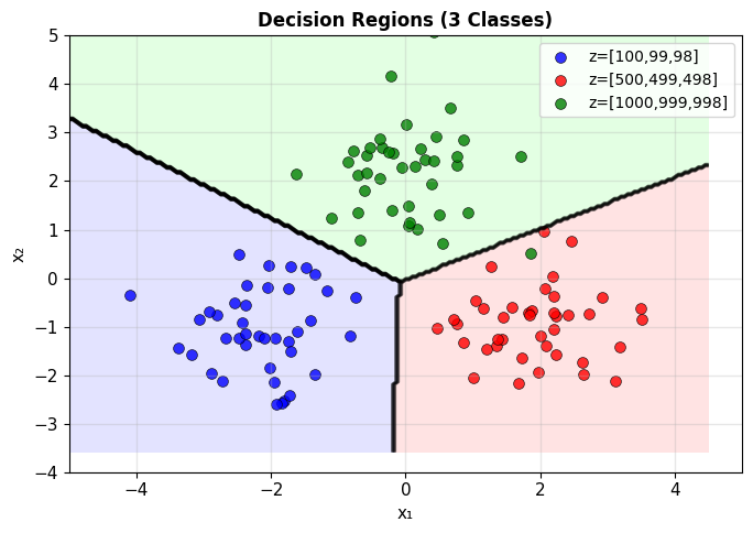
Each boundary is linear (hyperplane)
Cross-Entropy for Multi-Class
One-hot encoding for labels:
- Class 0: \(\mathbf{y} = [1, 0, 0]\)
- Class 1: \(\mathbf{y} = [0, 1, 0]\)
- Class 2: \(\mathbf{y} = [0, 0, 1]\)
Cross-entropy loss:
\[\mathcal{L} = -\sum_{k=1}^K y_k \log p_k\]
Since only one \(y_k = 1\):
\[\mathcal{L} = -\log p_{\text{true class}}\]
For entire dataset:
\[\text{NLL} = -\sum_{i=1}^n \log p_{i,y_i}\]
where \(p_{i,y_i}\) is predicted probability for true class of sample \(i\)
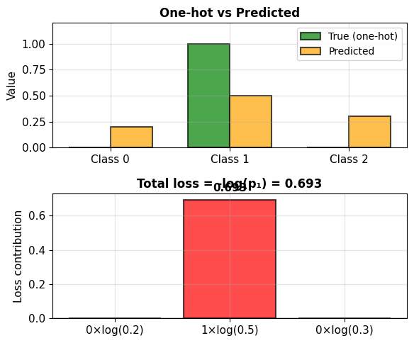
3-Class Softmax Computation
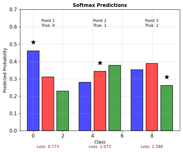
Data: 3 points, 3 classes
X = [[1, 0], [-1, 0], [0, 1]]
y = [0, 1, 2]  # Class labels
Current parameters:
W = [[0.5, 0.2, 0],    # w for class 0
     [0.1, 0.3, 0]]    # w for class 1,2
b = [0.1, 0, -0.1]
Computing predictions:
Point 1: \(\mathbf{x} = [1, 0]\)
- \(z_0 = 0.5(1) + 0.1(0) + 0.1 = 0.6\)
- \(z_1 = 0.2(1) + 0.3(0) + 0 = 0.2\)
- \(z_2 = 0(1) + 0(0) - 0.1 = -0.1\)
- \(\mathbf{p} = \text{softmax}([0.6, 0.2, -0.1]) = [0.47, 0.32, 0.21]\)
- True class: 0, Loss: \(-\log(0.47) = 0.76\)
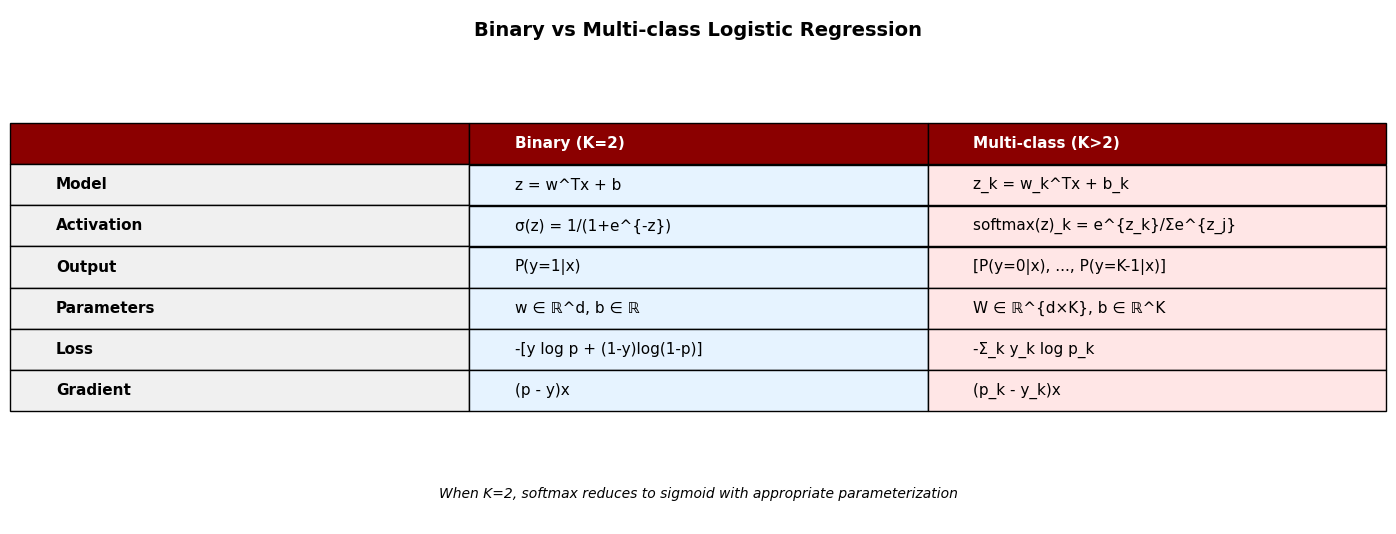
Binary to Multiclass – A Unified View
Separable Data Leads to Weight Explosion in MLE
Perfect separation scenario:
# 2D data with polynomial features
X = [[-2, -1], [-1, -2], [1, 2], [2, 1]]
y = [0, 0, 1, 1]
# Add polynomial features
X_poly = [[x1, x2, x1², x2², x1x2]
          for x1, x2 in X]
With 5 features for 4 points:
- Can achieve perfect separation
- MLE drives weights → ∞
- Predictions become 0 or 1 exactly
- No unique solution
The problem:
- Loss keeps decreasing: NLL → 0
- But weights explode: ||w|| → ∞
- Model becomes overconfident
- Poor generalization to new data
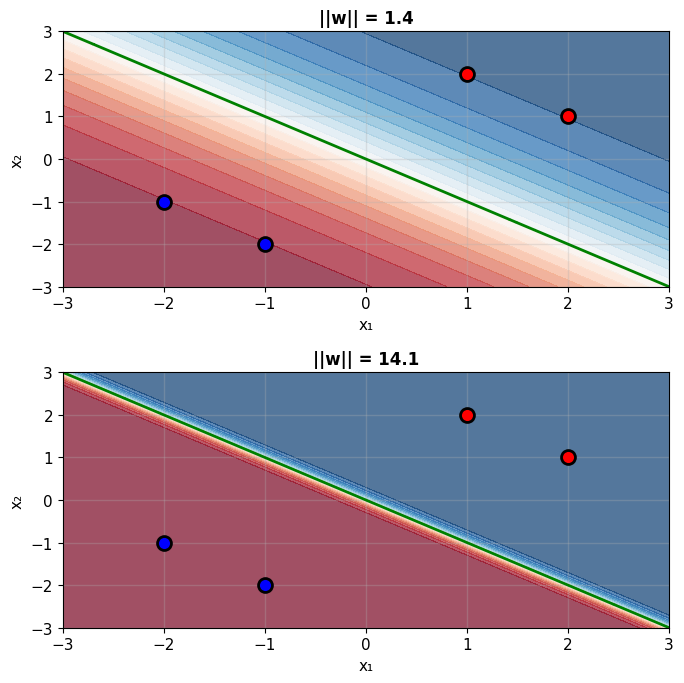
As ||w|| increases:
- Decision boundary sharpens
- Probabilities → 0 or 1
- Model becomes “too sure”
Weight Explosion in High Dimensions
Example: 100 features, 80 samples
Without regularization:
n, d = 80, 100  # More features than samples
X = np.random.randn(n, d)
y = (X @ w_true + noise > 0).astype(int)
What happens during optimization:
- Early iterations: Reasonable weights
- Middle: Some weights grow large
- Late: Many weights explode
- “Solution”: Perfect training accuracy
- But: Poor generalization (test performance)
Weight explosion occurs when:
- \(d > n\) (more features than samples)
- Features are highly correlated
- Perfect or near-perfect separation exists
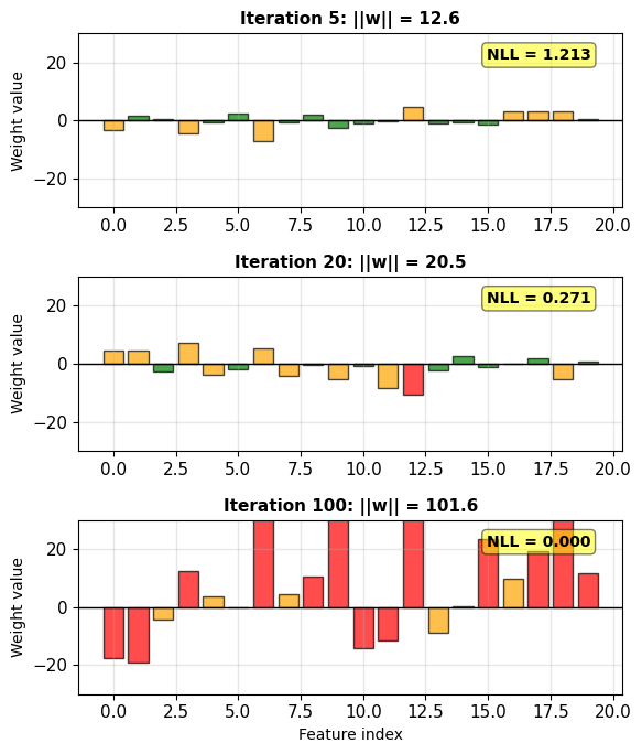
Loss decreases but weights are unstable.
Ridge (L2) Regularization Penalizes Large Weights
Modified objective:
\[\mathcal{L}_{\text{ridge}} = \underbrace{-\ell(\mathbf{w})}_{\text{NLL}} + \underbrace{\lambda ||\mathbf{w}||^2}_{\text{penalty}}\]
Gradient with regularization:
\[\nabla \mathcal{L}_{\text{ridge}} = -\mathbf{X}^T(\mathbf{y} - \mathbf{p}) + 2\lambda\mathbf{w}\]
Compare to unregularized:
\[\nabla \ell = \mathbf{X}^T(\mathbf{y} - \mathbf{p})\]
Effect: Pull weights toward zero
Update rule:
\[\mathbf{w} \leftarrow \mathbf{w} - \eta[\nabla \ell - 2\lambda\mathbf{w}]\]
\[= (1 - 2\eta\lambda)\mathbf{w} - \eta\nabla \ell\]
Weight decay: Shrink by factor \((1 - 2\eta\lambda)\)
L2 Regularization = Bias toward smaller weights.
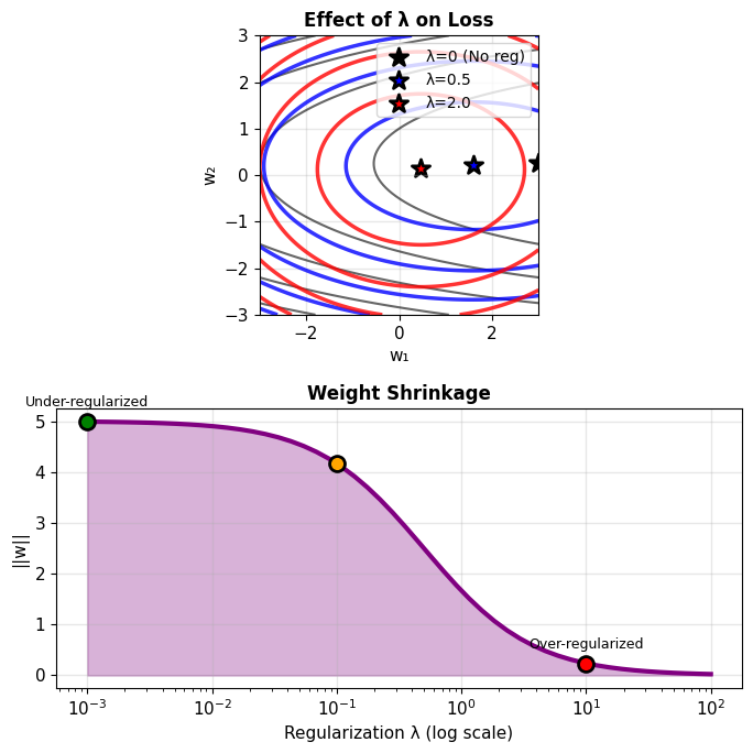
Larger λ → Smaller weights → More stable model
L2 Regularization = Gaussian Prior on Weights
L2 regularization = Gaussian prior
Prior on weights:
\[P(\mathbf{w}) = \mathcal{N}(\mathbf{0}, \sigma^2\mathbf{I})\]
\[\propto \exp\left(-\frac{||\mathbf{w}||^2}{2\sigma^2}\right)\]
MAP estimation:
\[\hat{\mathbf{w}}_{\text{MAP}} = \arg\max_\mathbf{w} P(\mathcal{D}|\mathbf{w})P(\mathbf{w})\]
Taking logarithm:
\[= \arg\max_\mathbf{w} \left[\log P(\mathcal{D}|\mathbf{w}) + \log P(\mathbf{w})\right]\]
\[= \arg\max_\mathbf{w} \left[\ell(\mathbf{w}) - \frac{||\mathbf{w}||^2}{2\sigma^2}\right]\]
With \(\lambda = \frac{1}{2\sigma^2}\):
\[= \arg\min_\mathbf{w} \left[-\ell(\mathbf{w}) + \lambda ||\mathbf{w}||^2\right]\]
This is Ridge regression
Smaller σ gives stronger regularization
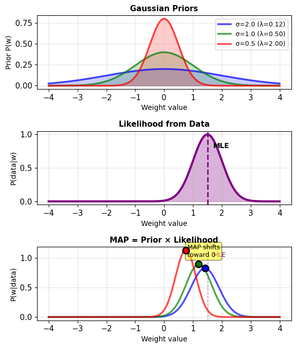
LASSO (L1) Regularization Drives Weights to Exactly Zero
LASSO (Least Absolute Shrinkage and Selection Operator)
L1 penalty:
\[\mathcal{L}_{\text{lasso}} = -\ell(\mathbf{w}) + \lambda ||\mathbf{w}||_1\]
\[= -\ell(\mathbf{w}) + \lambda \sum_{j=1}^d |w_j|\]
Subgradient (not differentiable at 0):
\[\partial_{w_j} \mathcal{L} = -\frac{\partial \ell}{\partial w_j} + \lambda \cdot \text{sign}(w_j)\]
where \(\text{sign}(w) = \begin{cases} +1 & w > 0 \\ [-1, 1] & w = 0 \\ -1 & w < 0 \end{cases}\)
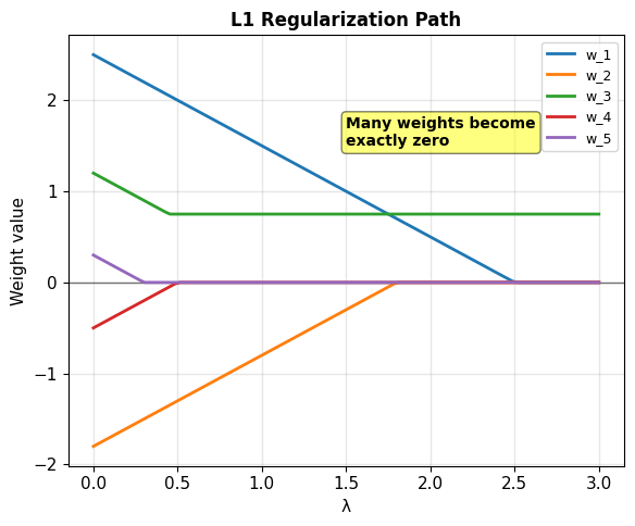
Induces exact sparsity: Many weights become exactly zero
Bayesian view: Laplace prior
\[P(\mathbf{w}) \propto \exp(-\lambda ||\mathbf{w}||_1)\]
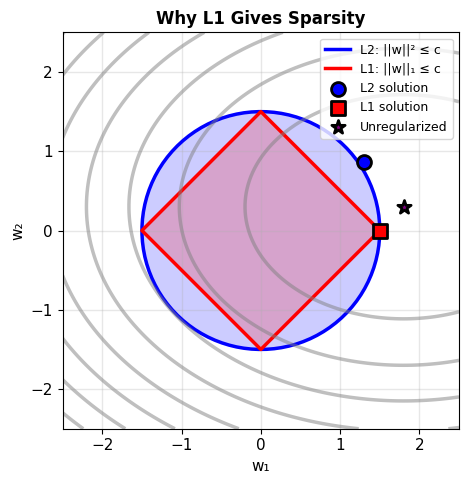
L1 hits corners → Some weights exactly 0
Elastic Net: Combined L1 and L2
Combine L1 and L2:
\[\mathcal{L}_{\text{elastic}} = -\ell(\mathbf{w}) + \lambda_1 ||\mathbf{w}||_1 + \lambda_2 ||\mathbf{w}||^2\]
Alternative parameterization:
\[= -\ell(\mathbf{w}) + \lambda\left[\alpha ||\mathbf{w}||_1 + \frac{1-\alpha}{2}||\mathbf{w}||^2\right]\]
where:
- \(\alpha = 1\): Pure L1 (Lasso)
- \(\alpha = 0\): Pure L2 (Ridge)
- \(0 < \alpha < 1\): Mix of both
Advantages:
- Sparsity from L1
- Grouping from L2 (correlated features)
- Stability when \(p > n\)
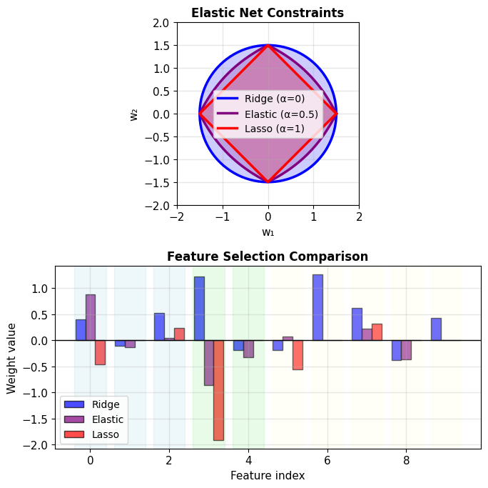
Elastic Net: Selects groups of correlated features
Choosing Regularization Strength (\(\lambda\)) by Cross-Validation
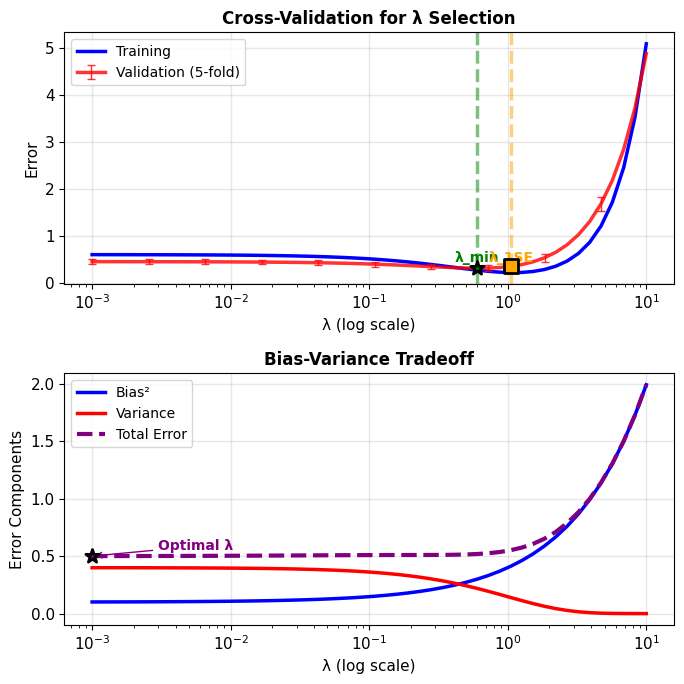
k-fold cross-validation:
-
Split data into \(k\) “folds”
-
For each \(\lambda\):
- Train on \(k-1\) folds
- Validate on remaining fold
- Repeat \(k\) times
-
Average validation error
-
Choose \(\lambda\) with lowest error
Common choices:
- \(k = 5\) or \(k = 10\)
- Leave-one-out: \(k = n\) (expensive)
One standard error rule:
- Find \(\lambda_{\text{min}}\) with minimum validation error
- Find largest \(\lambda\) within 1 standard error of minimum
- Choose simpler model (larger \(\lambda\)) when comparable
Larger λ within 1 SE yields simpler models with comparable performance
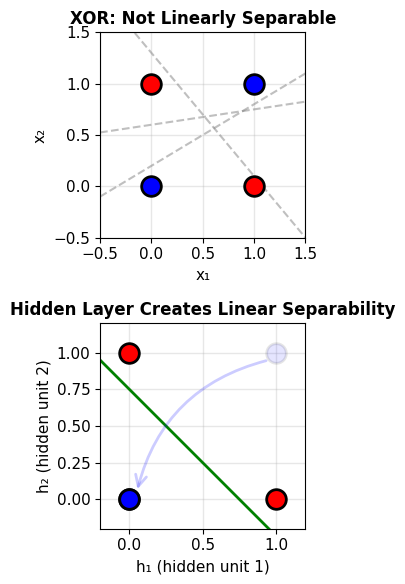
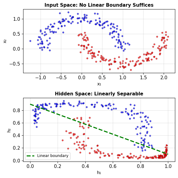
The “XOR Problem”
Linear decision boundaries cannot solve XOR.
XOR (Exclusive OR):
- (0,0) → Class 0 (blue)
- (0,1) → Class 1 (red)
- (1,0) → Class 1 (red)
- (1,1) → Class 0 (blue)
No linear boundary exists
Any line through the space:
- Misclassifies at least 2 points
- 50% accuracy at best
Logistic regression fails because:
\[P(y=1|\mathbf{x}) = \sigma(\mathbf{w}^T\mathbf{x} + b)\]
enforces linear decision boundary
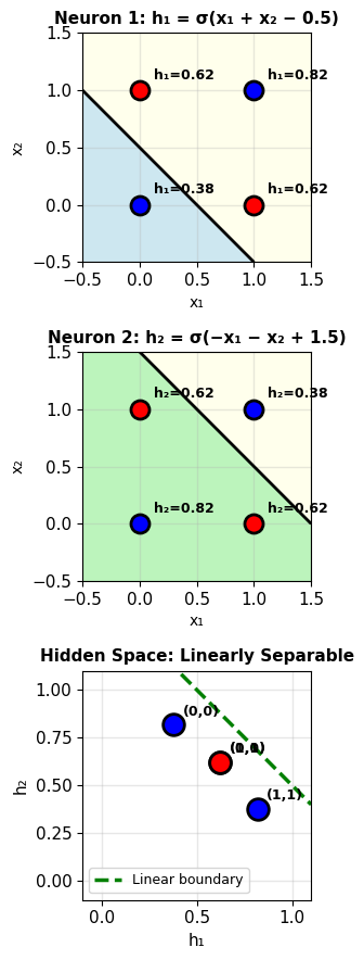
Solution: Add hidden layer
- Transform features nonlinearly
- Create linearly separable representation
- 2 hidden units sufficient for XOR
Logistic Regression Computes Exactly One Neuron’s Forward Pass
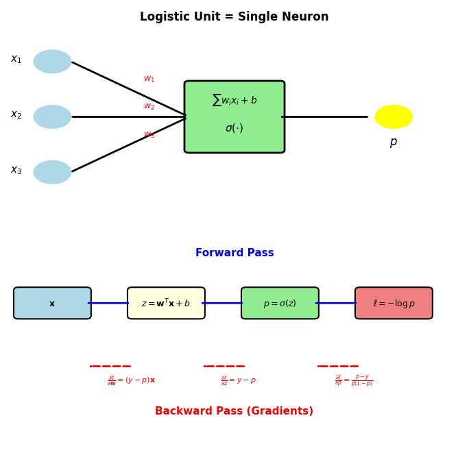
Same equations, different vocabulary:
| Logistic Regression | Neural Network |
|---|---|
| \(z = \mathbf{w}^T\mathbf{x} + b\) | pre-activation |
| \(p = \sigma(z)\) | activation |
| \(\mathcal{L} = -[y\log p + (1-y)\log(1-p)]\) | cross-entropy loss |
| \(\nabla_\mathbf{w}\ell = (y-p)\mathbf{x}\) | backpropagation (1 layer) |
Forward pass:
\[\mathbf{x} \to \mathbf{w}^T\mathbf{x} + b \to \sigma(\cdot) \to p\]
Backward pass (chain rule):
\[\frac{\partial \ell}{\partial \mathbf{w}} = \underbrace{(y - p)}_{\partial \ell / \partial z} \cdot \mathbf{x}\]
A single neuron with sigmoid activation is logistic regression. The gradient computation is backpropagation through one layer.
Stacking Neurons Creates Nonlinear Decision Boundaries
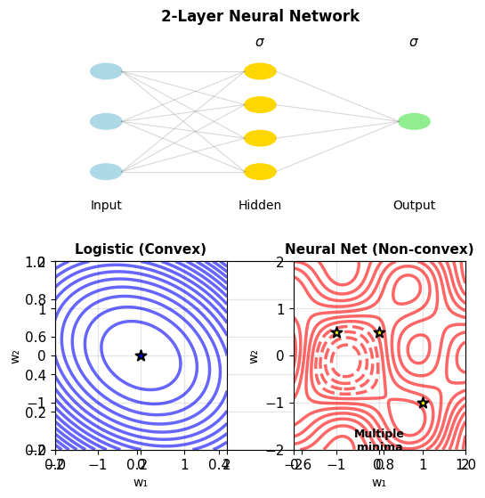
Two-layer network:
\[\mathbf{h} = \sigma(\mathbf{W}_1\mathbf{x} + \mathbf{b}_1)\]
\[p = \sigma(\mathbf{w}_2^T\mathbf{h} + b_2)\]
- \(\mathbf{W}_1 \in \mathbb{R}^{m \times d}\): first layer weights
- \(\mathbf{h} \in \mathbb{R}^m\): hidden representation
- \(\mathbf{w}_2 \in \mathbb{R}^m\): output layer weights
What stays the same:
- Cross-entropy loss
- Gradient = (error \(\times\) features), extended by chain rule
What changes:
- Hidden layer learns representation \(\mathbf{h}\) where data becomes linearly separable
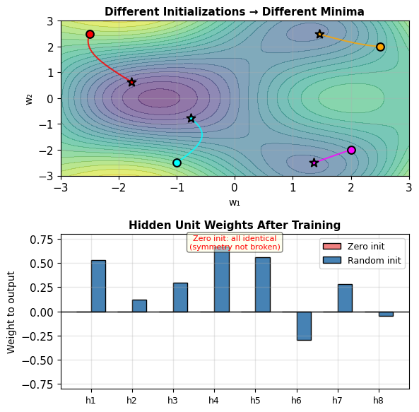
- Optimization is non-convex: multiple local minima, initialization matters
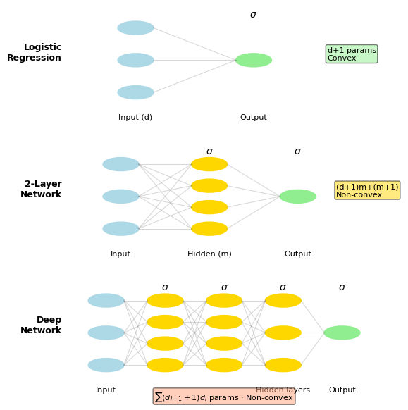
- Parameters: \((d+1)m + (m+1)\) vs \(d+1\) for logistic
Non-Convexity Means Initialization and Learning Rate Matter
Logistic regression (convex):
- Any starting point → global optimum
- Solution is unique (if \(\mathbf{X}\) full rank)
Neural networks (non-convex):
- Different initializations → different local minima
- Different minima → different generalization
Zero initialization breaks symmetry:
- All hidden units compute \(\sigma(\mathbf{0}^T\mathbf{x} + 0) = 0.5\)
- All receive identical gradients
- All learn the same function
- \(m\) hidden units collapse to 1
Random initialization:
- Breaks symmetry: each unit starts differently
- Scale matters: too large → saturation, too small → slow
Permutation symmetry: \(m\) hidden units → \(m!\) equivalent solutions from reordering alone
Adding Depth Changes Optimization, Not the Learning Principle
Logistic regression = neural network with 0 hidden layers
Adding layers:
- Same loss function (cross-entropy)
- Same gradient principle (chain rule extends naturally)
- New representational power: universal approximation with sufficient width
What breaks:
- Convex \(\to\) non-convex: no guarantee of global optimum
- Initialization matters (zero init causes symmetry problems)
- Multiple solutions with different generalization behavior
Parameter growth:
| Architecture | Parameters |
|---|---|
| Single neuron | \(d + 1\) |
| 1 hidden (\(m\) units) | \((d+1)m + (m+1)\) |
| \(L\) layers | \(\sum_{l=1}^{L} (d_{l-1}+1)d_l\) |