Theory Needs \(p(x,y)\), Practice Has Samples
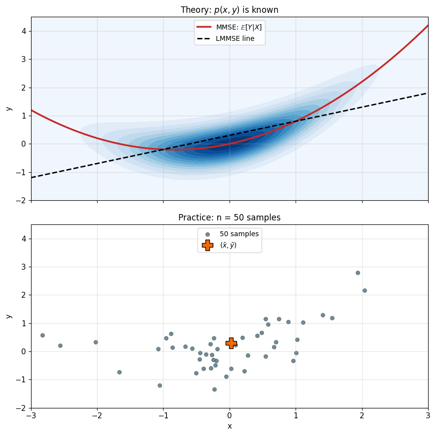
MMSE: \(\hat{Y} = \mathbb{E}[Y|X]\)
- Requires \(p(y|x)\) to compute conditional expectation
Linear MMSE: \(\hat{Y} = \frac{\text{Cov}(X,Y)}{\text{Var}(X)}(X - \mathbb{E}[X]) + \mathbb{E}[Y]\)
- Requires population moments: \(\mathbb{E}[X]\), \(\mathbb{E}[Y]\), Var\((X)\), Cov\((X,Y)\)
In practice:
- Don’t know distributions
- Don’t know population moments
- Only have finite samples: \((x_1, y_1), ..., (x_n, y_n)\)
Empirical approximation:
\[\mathbb{E}[h(X)] \approx \frac{1}{n}\sum_{i=1}^n h(x_i)\]
\[\text{Cov}(X,Y) \approx \frac{1}{n}\sum_{i=1}^n (x_i - \bar{x})(y_i - \bar{y})\]
Sample Averages Converge to Population Averages
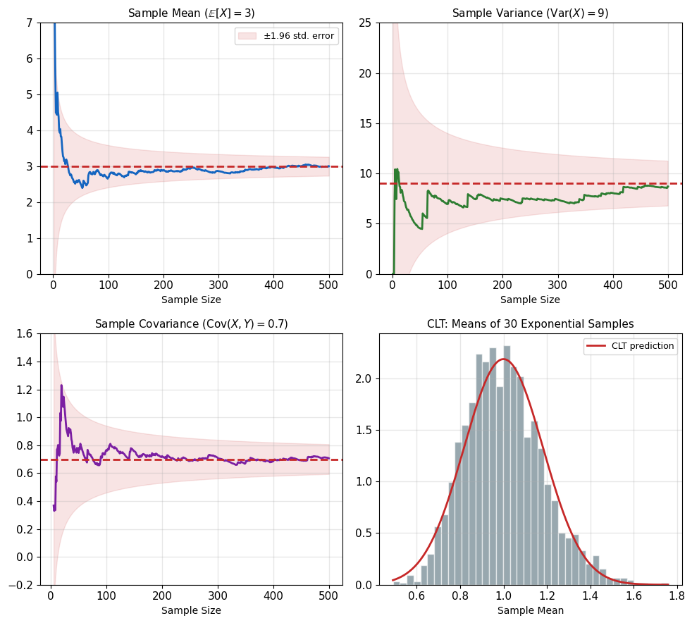
Population moments – require \(p(x)\):
\[\mathbb{E}[X] = \int x \cdot p(x) \, dx\]
\[\text{Var}(X) = \int (x - \mathbb{E}[X])^2 p(x) \, dx\]
Sample moments – require only data:
\[\bar{X} = \frac{1}{n} \sum_{i=1}^n X_i, \qquad S_X^2 = \frac{1}{n} \sum_{i=1}^n (X_i - \bar{X})^2\]
Law of Large Numbers: \(\bar{X} \xrightarrow{a.s.} \mathbb{E}[X]\)
Central Limit Theorem: \(\sqrt{n}(\bar{X} - \mathbb{E}[X]) \xrightarrow{d} \mathcal{N}(0, \text{Var}(X))\)
- Error shrinks as \(1/\sqrt{n}\)
Monte Carlo approximation: integrals become sums over samples
ERM Minimizes the Computable Risk
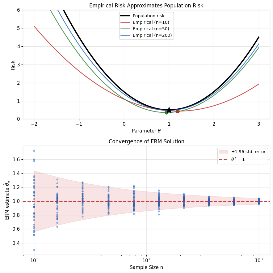
Population risk (what we want to minimize):
\[R(f) = \mathbb{E}_{(X,Y)}[\ell(Y, f(X))]\]
\[= \int\int \ell(y, f(x)) \, p(x,y) \, dx \, dy\]
Cannot compute without knowing \(p(x,y)\)
Empirical risk (what we can compute):
\[\hat{R}_n(f) = \frac{1}{n} \sum_{i=1}^n \ell(y_i, f(x_i))\]
Empirical Risk Minimization (ERM):
\[\hat{f}_n = \arg\min_{f \in \mathcal{F}} \hat{R}_n(f)\]
Convergence guarantee (fixed \(\mathcal{F}\), not too rich):
\[R(\hat{f}_n) - \inf_{f \in \mathcal{F}} R(f) \xrightarrow{P} 0\]
Risk of the sample minimizer approaches the best risk in \(\mathcal{F}\)
Training Error Underestimates Risk
Training error: \(\hat{R}_n(\hat{f}_n)\), the empirical risk of the fit on the data that produced it
Test error: \(\hat{R}(\hat{f}_n)\) on held-out data, an unbiased estimate of \(R(\hat{f}_n)\)
The order never changes (\(f^*\) the best in \(\mathcal{F}\)):
\[\mathbb{E}[\hat{R}_n(\hat{f}_n)] \leq R(f^*) \leq \mathbb{E}[R(\hat{f}_n)]\]
- Left: \(\hat{f}_n\) was chosen to make \(\hat{R}_n\) small
- Right: \(f^*\) is the best on the population, \(\hat{f}_n\) is not
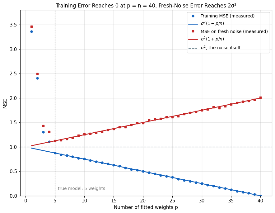
Least squares, \(p\) weights, \(n\) samples, noise variance \(\sigma^2\):
- \(\mathbb{E}[\text{training MSE}] = \sigma^2(1 - p/n)\)
- \(\mathbb{E}[\text{MSE on fresh noise at the same inputs}] = \sigma^2(1 + p/n)\)
- \(p = n\): training error 0, the fit interpolates the noise
Overfitting: the gap \(2\sigma^2 p/n\) grows with every added weight
The Loss Encodes the Noise Model
ERM: Minimize a loss over data
\[\hat{f} = \arg\min_{f} \frac{1}{n}\sum_{i=1}^n \ell(y_i, f(x_i))\]
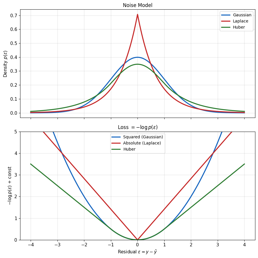
Which loss? Different choices give different estimators:
- Squared: \((y - \hat{y})^2\)
- Absolute: \(|y - \hat{y}|\)
- Huber: squared near zero, absolute in the tails
The choice encodes assumptions about how noise enters the data
Maximum likelihood makes this explicit:
- Specify a probabilistic model for data generation
- The loss function emerges from the model
- Different noise gives a different loss
Data = Linear Signal + Random Noise
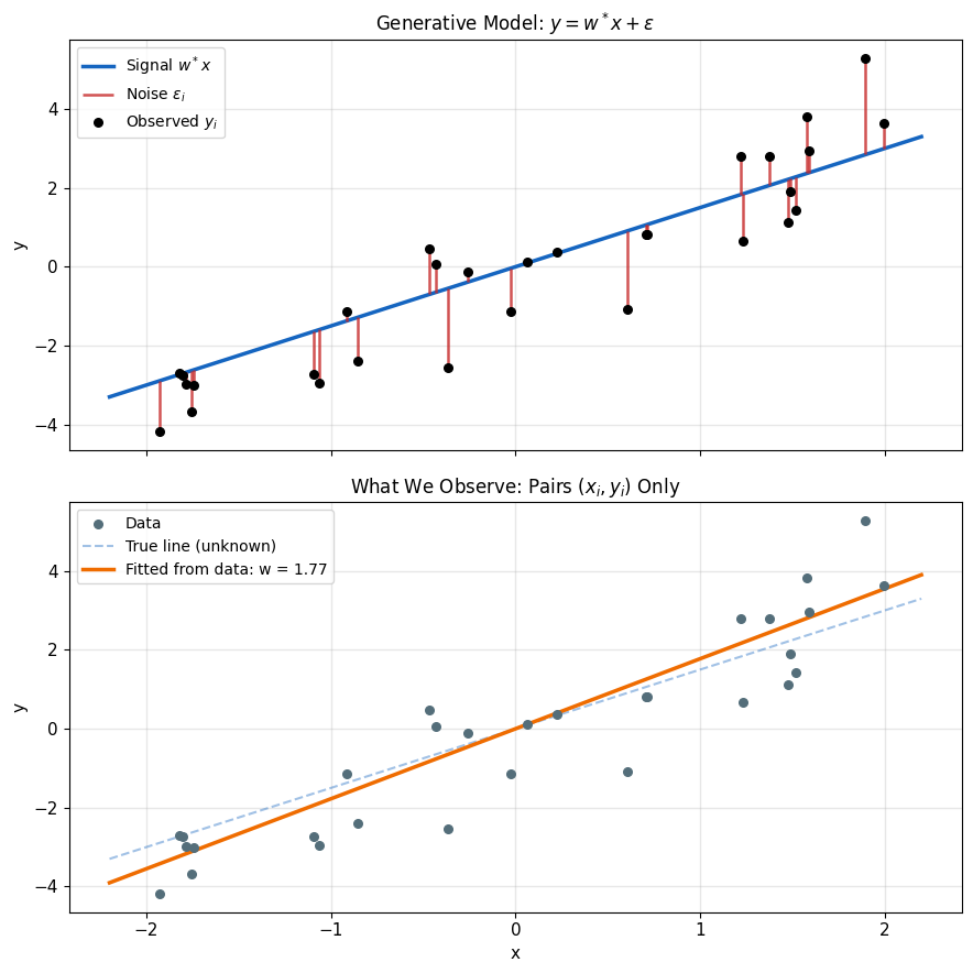
Assume data comes from a process:
\[y = \mathbf{w}^T \mathbf{x} + \epsilon\]
where \(\epsilon\) is random noise (\(\mathbf{x}\) includes a constant 1, so the bias is in \(\mathbf{w}\))
What we observe:
- Pairs \((\mathbf{x}_i, y_i)\)
- Never \(\mathbf{w}^T \mathbf{x}_i\) and \(\epsilon_i\) separately
Questions:
- What distribution for \(\epsilon\)?
- How does this affect estimation?
Common assumption: \(\epsilon \sim \mathcal{N}(0, \sigma^2)\)
Why Gaussian? Often reasonable in practice:
- Central limit theorem: sum of many small effects
- Maximum entropy for fixed variance
- Mathematical tractability
The Noise Model Defines the Likelihood
Model: \(y = \mathbf{w}^T \mathbf{x} + \epsilon\), where \(\epsilon \sim \mathcal{N}(0, \sigma^2)\)
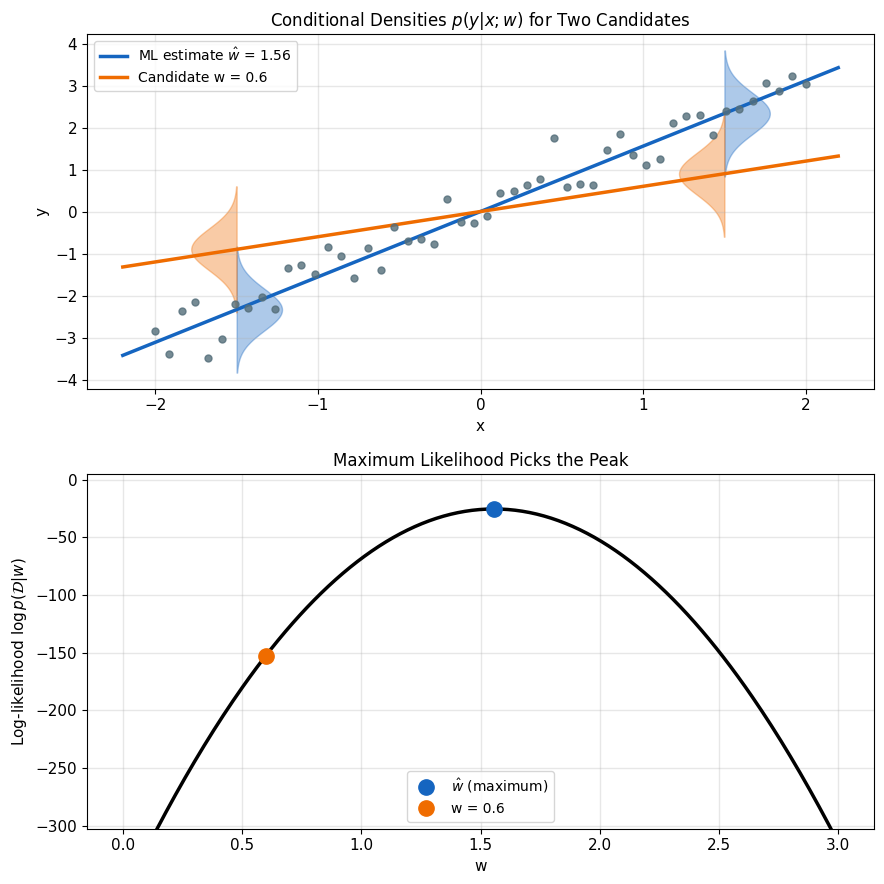
This implies \(y|\mathbf{x}\) is Gaussian:
\[y|\mathbf{x} \sim \mathcal{N}(\mathbf{w}^T \mathbf{x}, \sigma^2)\]
Density of \(y\) given \(\mathbf{x}\):
\[p(y|\mathbf{x}; \mathbf{w}) = \frac{1}{\sqrt{2\pi\sigma^2}} \exp\left(-\frac{(y - \mathbf{w}^T \mathbf{x})^2}{2\sigma^2}\right)\]
For entire dataset \(\mathcal{D} = \{(\mathbf{x}_i, y_i)\}_{i=1}^n\):
Assuming independent samples:
\[p(\mathcal{D}|\mathbf{w}) = \prod_{i=1}^n p(y_i|\mathbf{x}_i; \mathbf{w})\]
Maximum likelihood principle: Find \(\mathbf{w}\) that makes observed data most likely:
\[\hat{\mathbf{w}}_{\text{ML}} = \arg\max_{\mathbf{w}} p(\mathcal{D}|\mathbf{w})\]
Equivalently, minimize \(-\frac{1}{n}\sum_i \log p(y_i|\mathbf{x}_i; \mathbf{w})\): ERM with loss \(\ell = -\log p\)
From Likelihood to Least Squares
Log-likelihood:
\[\log L(\mathbf{w}) = \log p(\mathcal{D}|\mathbf{w}) = \sum_{i=1}^n \log p(y_i|\mathbf{x}_i; \mathbf{w})\]
Substitute Gaussian pdf:
\[\log L(\mathbf{w}) = \sum_{i=1}^n \log \left(\frac{1}{\sqrt{2\pi\sigma^2}} e^{-\frac{(y_i - \mathbf{w}^T \mathbf{x}_i)^2}{2\sigma^2}}\right)\]
Simplify:
\[\log L(\mathbf{w}) = -\frac{n}{2}\log(2\pi\sigma^2) - \frac{1}{2\sigma^2}\sum_{i=1}^n(y_i - \mathbf{w}^T \mathbf{x}_i)^2\]
To maximize \(\log L(\mathbf{w})\):
- First term: constant w.r.t. \(\mathbf{w}\)
- Second term: minimize \(\sum_i(y_i - \mathbf{w}^T \mathbf{x}_i)^2\)
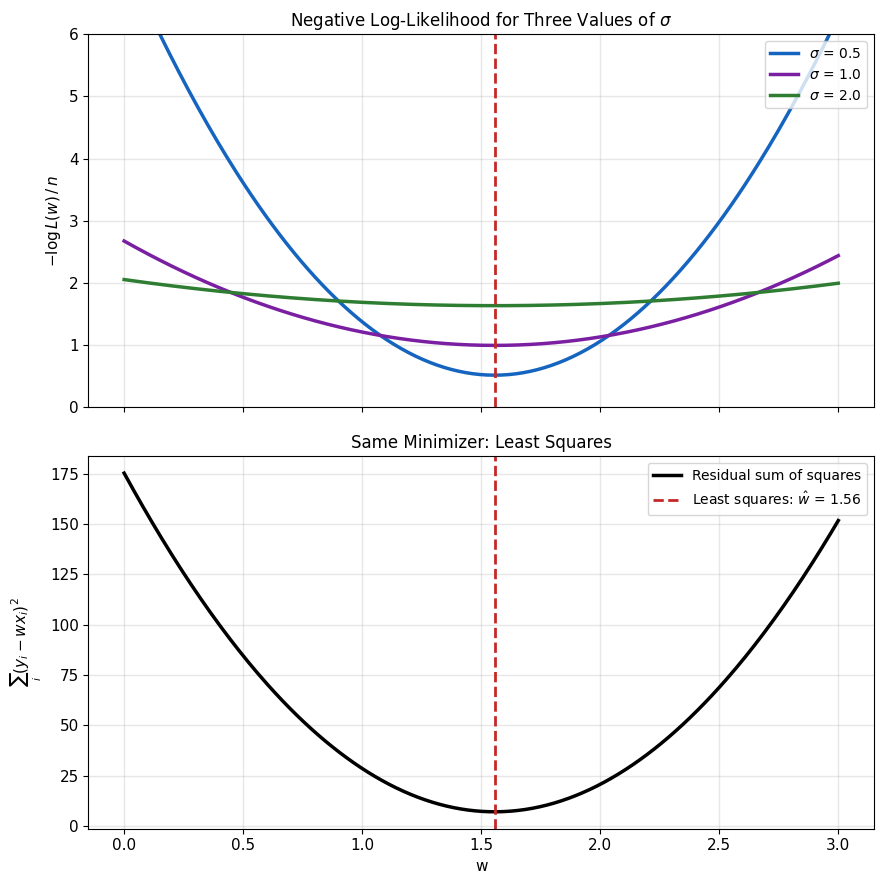
Result: MLE = Least squares
\[\hat{\mathbf{w}}_{\text{ML}} = \arg\min_{\mathbf{w}} \sum_{i=1}^n(y_i - \mathbf{w}^T \mathbf{x}_i)^2\]
Gaussian noise assumption leads to squared loss
Laplace Noise Gives Least Absolute Deviations
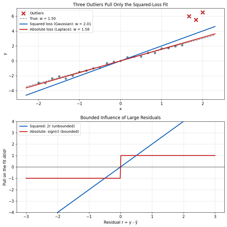
Real data has outliers:
- Sensor errors
- Data entry mistakes
- Rare events
Laplace noise model:
\[p(\epsilon) = \frac{1}{2b}\exp\left(-\frac{|\epsilon|}{b}\right)\]
Heavier tails than Gaussian: large residuals are not unusual
Likelihood with Laplace noise:
\[p(y|\mathbf{x}; \mathbf{w}) = \frac{1}{2b}\exp\left(-\frac{|y - \mathbf{w}^T \mathbf{x}|}{b}\right)\]
Log-likelihood:
\[\log L(\mathbf{w}) = -n\log(2b) - \frac{1}{b}\sum_{i=1}^n |y_i - \mathbf{w}^T \mathbf{x}_i|\]
Maximizing \(\log L(\mathbf{w})\) equivalent to minimizing:
\[\sum_{i=1}^n |y_i - \mathbf{w}^T \mathbf{x}_i|\]
L1 loss emerges directly from the Laplace noise assumption.
This is least absolute deviations (LAD): the fit tracks the conditional median, not the mean
- Not Lasso: Lasso keeps squared loss and adds an L1 penalty on \(\mathbf{w}\)
Residual Structure Exposes Bad Assumptions
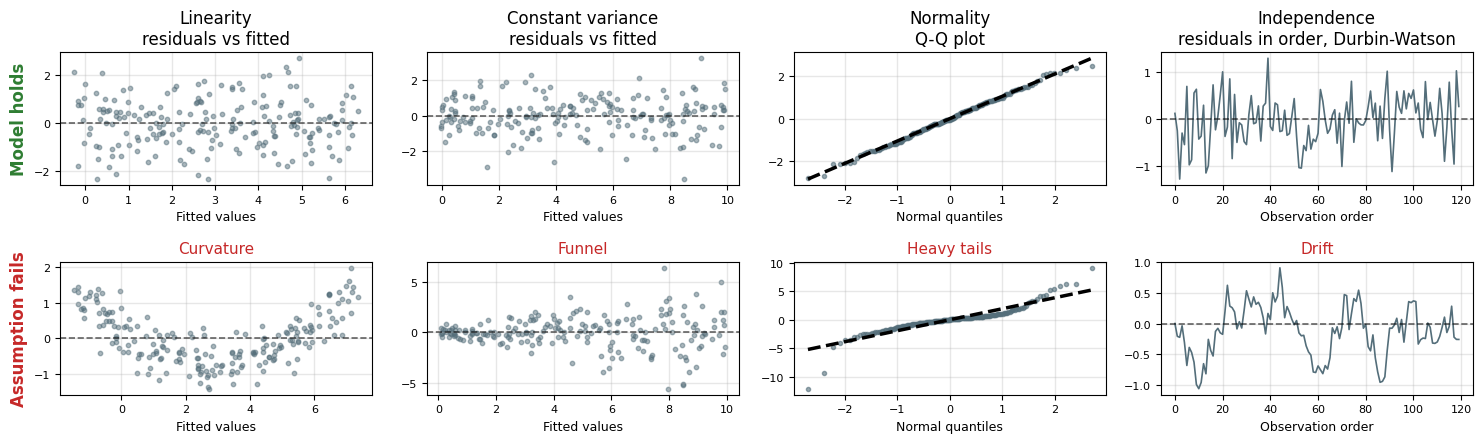
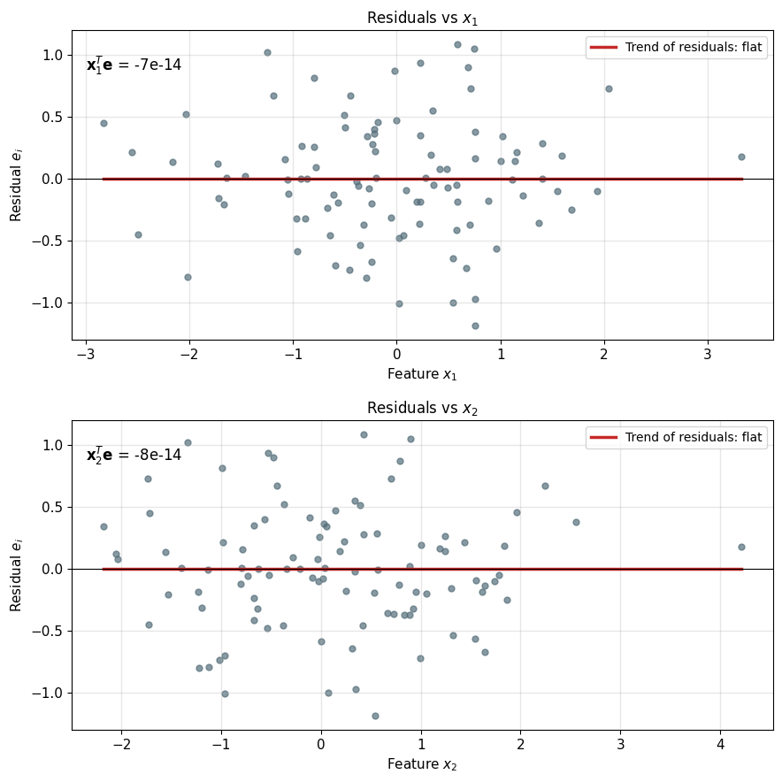
Residuals \(e_i = y_i - \hat{y}_i\) estimate the noise: each plot tests one part of \(\epsilon_i \sim \mathcal{N}(0, \sigma^2)\), independent
When linear regression fails:
- Nonlinear relationships: polynomial/nonlinear models
- Non-constant variance: transform response or weighted regression
- Heavy-tailed errors: absolute (LAD) or Huber loss
- Correlated errors: time series models
The Bias Becomes One More Weight
Notation: Weight vector \(\mathbf{w}\), bias \(b\) (replacing LMMSE parameters \(\mathbf{a}, b\))
Model structure:
\[\hat{y} = \mathbf{w}^T \mathbf{x} + b\]
where:
- \(\mathbf{x} \in \mathbb{R}^p\): feature vector
- \(\mathbf{w} \in \mathbb{R}^p\): weight vector
- \(b \in \mathbb{R}\): bias/intercept
- \(\hat{y} \in \mathbb{R}\): prediction
Vectorized over dataset:
\[\hat{\mathbf{y}} = \mathbf{X}\mathbf{w} + b\mathbf{1}\]
- \(\mathbf{X} \in \mathbb{R}^{n \times p}\): data matrix
- \(\mathbf{y} \in \mathbb{R}^n\): target vector
- \(\mathbf{1} \in \mathbb{R}^n\): vector of ones
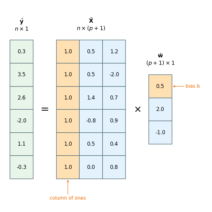
Augmented notation (absorb the bias):
\[\tilde{\mathbf{x}} = \begin{bmatrix} 1 \\ \mathbf{x} \end{bmatrix}, \quad \tilde{\mathbf{w}} = \begin{bmatrix} b \\ \mathbf{w} \end{bmatrix}\]
Then: \(\hat{y} = \tilde{\mathbf{w}}^T \tilde{\mathbf{x}}\) and \(\hat{\mathbf{y}} = \tilde{\mathbf{X}}\tilde{\mathbf{w}}\). From here on \(\mathbf{X}\) includes the column of ones.
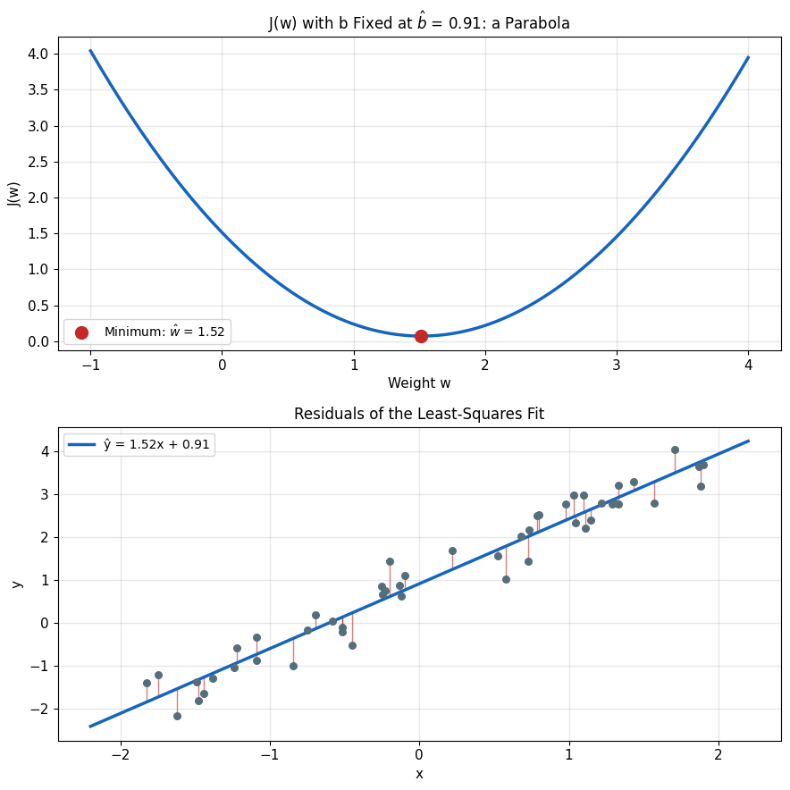
Least Squares Is a Quadratic in \(\mathbf{w}\)
Empirical risk (squared loss):
\[J(\mathbf{w}) = \frac{1}{2n} \sum_{i=1}^n (y_i - \underbrace{\mathbf{w}^T \mathbf{x}_i}_{\hat{y}_i})^2\]
Matrix form:
\[J(\mathbf{w}) = \frac{1}{2n} \|\mathbf{y} - \mathbf{X}\mathbf{w}\|^2\]
Expanded:
\[J(\mathbf{w}) = \frac{1}{2n}(\mathbf{y} - \mathbf{X}\mathbf{w})^T(\mathbf{y} - \mathbf{X}\mathbf{w})\]
\[= \frac{1}{2n}(\mathbf{y}^T\mathbf{y} - 2\mathbf{y}^T\mathbf{X}\mathbf{w} + \mathbf{w}^T\mathbf{X}^T\mathbf{X}\mathbf{w})\]
This is a quadratic in \(\mathbf{w}\):
\[J(\mathbf{w}) = \frac{1}{2n}(\mathbf{w}^T\mathbf{A}\mathbf{w} - 2\mathbf{c}^T\mathbf{w} + \mathbf{y}^T\mathbf{y})\]
where:
- \(\mathbf{A} = \mathbf{X}^T\mathbf{X}\) (always positive semidefinite)
- \(\mathbf{c} = \mathbf{X}^T\mathbf{y}\)
Convexity: \(\nabla^2 J = \frac{1}{n}\mathbf{X}^T\mathbf{X} \succeq 0\)
- \(\succeq 0\): positive semidefinite, \(\mathbf{v}^T (\nabla^2 J) \mathbf{v} \geq 0\) for every \(\mathbf{v}\)
- Curvature never negative in any direction, so every local minimum is global
Zero Gradient Makes Residuals Orthogonal to \(\mathbf{X}\)
Minimize: \(J(\mathbf{w}) = \frac{1}{2n}\|\mathbf{y} - \mathbf{X}\mathbf{w}\|^2\)
Take gradient:
\[\nabla_{\mathbf{w}} J = \frac{1}{n}\mathbf{X}^T(\mathbf{X}\mathbf{w} - \mathbf{y})\]
Set to zero:
\[\mathbf{X}^T(\mathbf{X}\mathbf{w} - \mathbf{y}) = \mathbf{0}\]
Normal equations:
\[\boxed{\mathbf{X}^T\mathbf{X}\mathbf{w} = \mathbf{X}^T\mathbf{y}}\]
Observations:
- \(\mathbf{X}^T\mathbf{X} \in \mathbb{R}^{p \times p}\): Gram matrix
- \(\mathbf{X}^T\mathbf{y} \in \mathbb{R}^p\): cross-correlation
- System is \(p\) equations in \(p\) unknowns
- Unique solution if \(\mathbf{X}^T\mathbf{X}\) invertible
Hence name: residual \(\mathbf{y} - \mathbf{X}\hat{\mathbf{w}}\) is orthogonal (normal) to every column of \(\mathbf{X}\) - the sample form of the orthogonality principle
Normal Equations Are the Sample LMMSE Equations
Normal equations: \(\mathbf{X}^T\mathbf{X}\mathbf{w} = \mathbf{X}^T\mathbf{y}\)
Divide by \(n\):
\[\frac{1}{n}\mathbf{X}^T\mathbf{X}\mathbf{w} = \frac{1}{n}\mathbf{X}^T\mathbf{y}\]
With the column of ones: \(\frac{1}{n}\mathbf{X}^T\mathbf{X}\) holds second moments, not covariances
Center first (\(\mathbf{X}_c\): each column minus its mean, \(\mathbf{y}_c = \mathbf{y} - \bar{y}\)): the ones column drops out and the equations become
\[\hat{\mathbf{K}}_{XX} \mathbf{w} = \hat{\mathbf{k}}_{XY}\]
- \(\hat{\mathbf{K}}_{XX} = \frac{1}{n}\mathbf{X}_c^T\mathbf{X}_c\): sample covariance matrix
- \(\hat{\mathbf{k}}_{XY} = \frac{1}{n}\mathbf{X}_c^T\mathbf{y}_c\): sample cross-covariance
- \(b = \bar{y} - \mathbf{w}^T\bar{\mathbf{x}}\) recovers the intercept
Solution:
\[\mathbf{w} = \hat{\mathbf{K}}_{XX}^{-1} \hat{\mathbf{k}}_{XY}\]
This is empirical LMMSE.
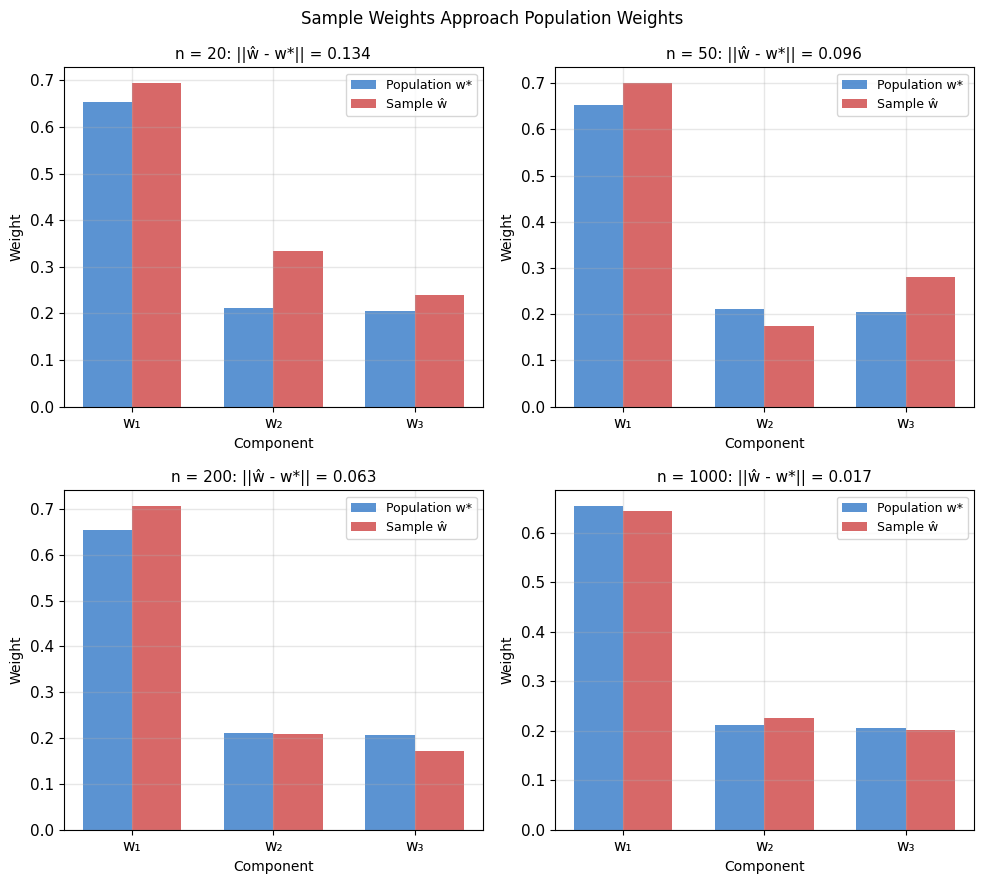
Population: \(\mathbf{w}^* = \mathbf{K}_{XX}^{-1} \mathbf{k}_{XY}\) Sample: \(\hat{\mathbf{w}} = \hat{\mathbf{K}}_{XX}^{-1} \hat{\mathbf{k}}_{XY}\)
Consistency: \(\hat{\mathbf{w}} \to \mathbf{w}^*\) as \(n \to \infty\)
Full Column Rank Gives a Unique Solution
Solution (when \(\mathbf{X}^T\mathbf{X}\) invertible):
\[\mathbf{w} = (\mathbf{X}^T\mathbf{X})^{-1}\mathbf{X}^T\mathbf{y}\]
Moore-Penrose pseudoinverse (full column rank):
\[\mathbf{X}^+ = (\mathbf{X}^T\mathbf{X})^{-1}\mathbf{X}^T\]
So: \(\mathbf{w} = \mathbf{X}^+\mathbf{y}\)
Properties of \(\mathbf{X}^+\):
- \(\mathbf{X}^+\mathbf{X} = \mathbf{I}_p\) (left inverse)
- \(\mathbf{X}\mathbf{X}^+ = \mathbf{P}_X\) (projection onto col(\(\mathbf{X}\)))
When is \(\mathbf{X}^T\mathbf{X}\) invertible?
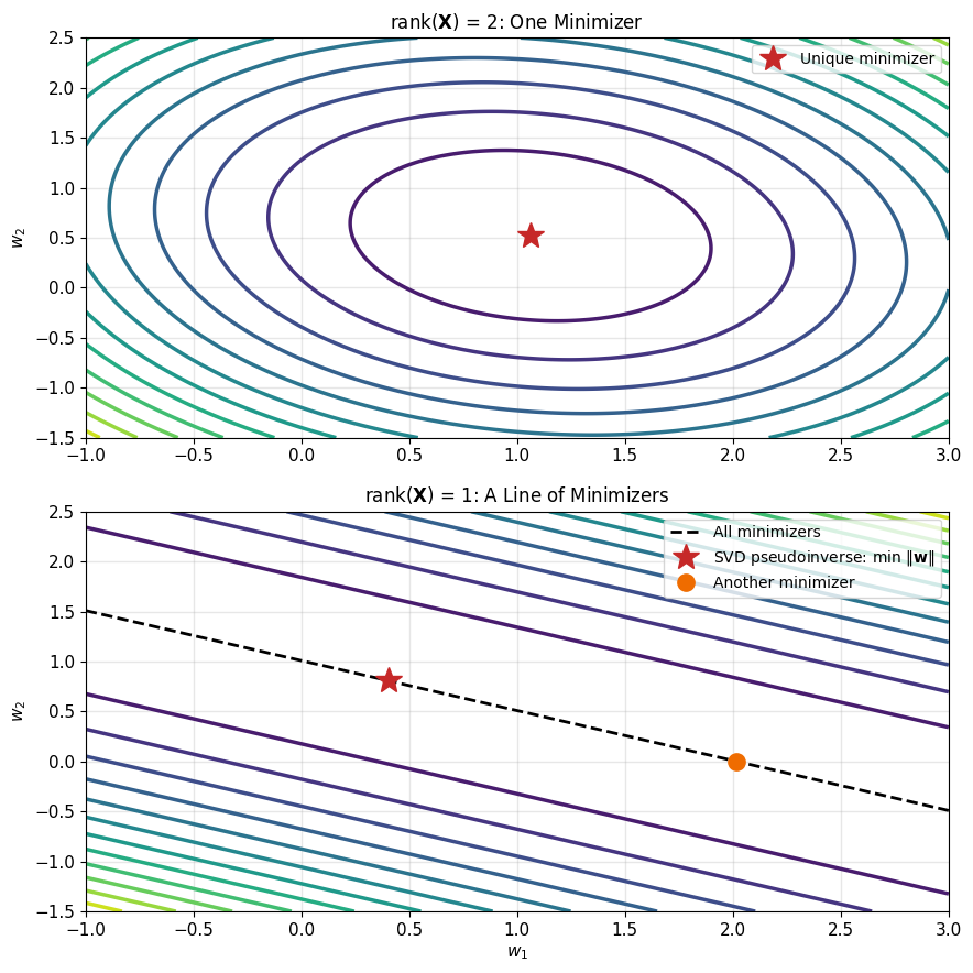
- Need \(\text{rank}(\mathbf{X}) = p\) (full column rank)
- Requires \(n \geq p\) (more data than features)
- Columns of \(\mathbf{X}\) linearly independent
Rank deficient case: infinitely many solutions; the SVD pseudoinverse picks the one with minimum \(\|\mathbf{w}\|\)
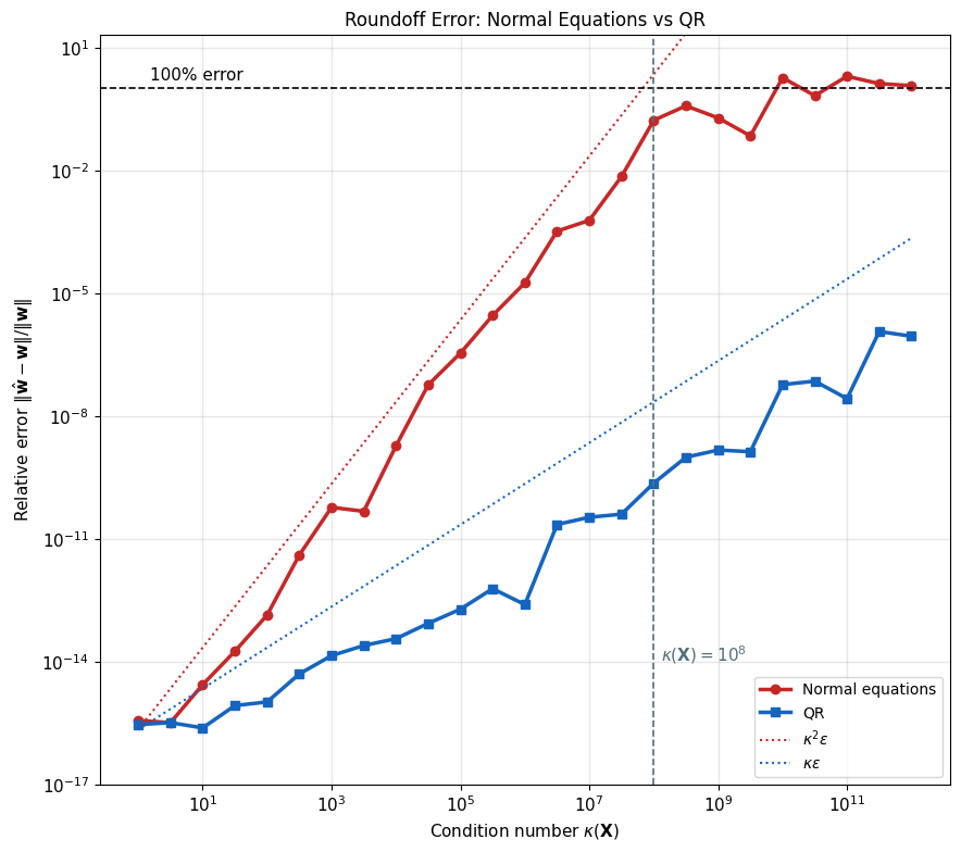
Computing \(\mathbf{X}^T\mathbf{X}\) Squares the Condition Number
Method 1: Normal equations
w = np.linalg.solve(X.T @ X, X.T @ y)
Complexity:
- Form \(\mathbf{X}^T\mathbf{X}\): \(O(np^2)\)
- Form \(\mathbf{X}^T\mathbf{y}\): \(O(np)\)
- Solve system: \(O(p^3)\)
- Total: \(O(np^2 + p^3)\), about \(np^2 + p^3/3\) flops
Condition number: \(\kappa(\mathbf{A}) = \sigma_{\max}(\mathbf{A}) / \sigma_{\min}(\mathbf{A})\), the ratio of largest to smallest singular value
- The largest factor by which solving with \(\mathbf{A}\) amplifies a relative error in the data
- For \(\mathbf{X}^T\mathbf{X}\): \(\lambda_{\max} / \lambda_{\min}\) of its eigenvalues (lecture 03’s \(\mathbf{K}_{XX}\))
Squaring:
\[\kappa(\mathbf{X}^T\mathbf{X}) = \kappa(\mathbf{X})^2\]
- Squaring doubles the digits lost
- float64 carries ~16 digits: at \(\kappa(\mathbf{X}) = 10^8\), none survive
SVD Handles Rank Deficiency
Singular Value Decomposition:
\[\mathbf{X} = \mathbf{U}\boldsymbol{\Sigma}\mathbf{V}^T\]
where:
- \(\mathbf{U} \in \mathbb{R}^{n \times p}\): orthonormal columns (left singular vectors)
- \(\boldsymbol{\Sigma} \in \mathbb{R}^{p \times p}\): diagonal, \(\sigma_1 \geq \cdots \geq \sigma_p \geq 0\)
- \(\mathbf{V} \in \mathbb{R}^{p \times p}\): orthogonal (right singular vectors)
Solution via SVD:
\[\mathbf{w} = \mathbf{V}\boldsymbol{\Sigma}^+ \mathbf{U}^T \mathbf{y}\]
where \(\boldsymbol{\Sigma}^+\) = pseudoinverse of \(\boldsymbol{\Sigma}\):
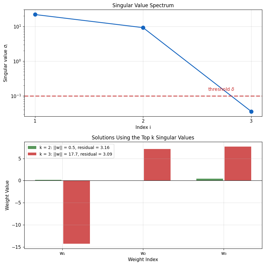
- If \(\sigma_i > \delta\): \(\sigma_i^+ = 1/\sigma_i\)
- If \(\sigma_i \leq \delta\): \(\sigma_i^+ = 0\)
Rank deficient: smallest \(\|\mathbf{w}\|\) among all minimizers
Component form: one term per singular direction
\[\hat{\mathbf{w}} = \sum_i f_i \, \frac{\mathbf{u}_i^T \mathbf{y}}{\sigma_i} \, \mathbf{v}_i, \qquad f_i \in \{0, 1\}\]
- Small \(\sigma_i\) divides: that direction carries the noise
- The filter factor \(f_i\) keeps or drops each direction whole
Cost:
- About \(2np^2 + 11p^3\) flops, the most of the three
np.linalg.lstsquses the SVD
Truncated SVD (regularization): \(f_i = 1\) for the \(k\) largest \(\sigma_i\), else \(0\)
- Ridge replaces the 0/1 switch by a smooth factor between them
Steepest Descent Moves Along \(-\nabla J\)
First-order Taylor expansion:
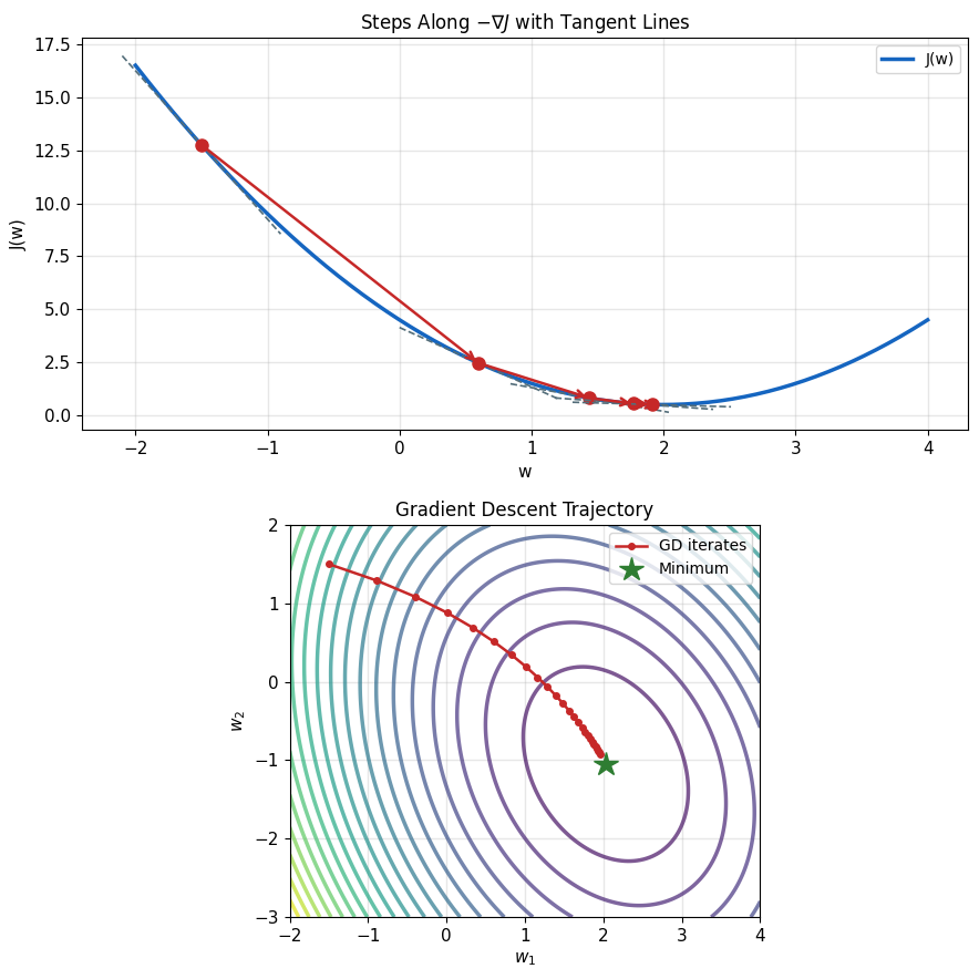
\[J(\mathbf{w} + \Delta) \approx J(\mathbf{w}) + \nabla J(\mathbf{w})^T\Delta\]
- For a fixed step length, the decrease is largest at \(\Delta \propto -\nabla J(\mathbf{w})\)
Gradient points uphill:
\[\nabla J(\mathbf{w}) = \frac{1}{n}\mathbf{X}^T(\mathbf{X}\mathbf{w} - \mathbf{y})\]
Direction of maximum increase of \(J\)
Update rule:
\[\mathbf{w}_{t+1} = \mathbf{w}_t - \eta \nabla J(\mathbf{w}_t)\]
where \(\eta\) = step size / learning rate
Convergence criterion:
\[\|\nabla J(\mathbf{w})\| < \text{tol}\]
At optimum: \(\nabla J(\mathbf{w}^*) = \mathbf{0}\) (critical point)
NumPy (\(\mathbf{X}\) includes the ones column):
def gradient_descent(X, y, eta=0.01, steps=1000):
    n, p = X.shape
    w = np.zeros(p)
    for _ in range(steps):
        grad = X.T @ (X @ w - y) / n
        w = w - eta * grad
    return w
Squared Loss Has No Bad Local Minima
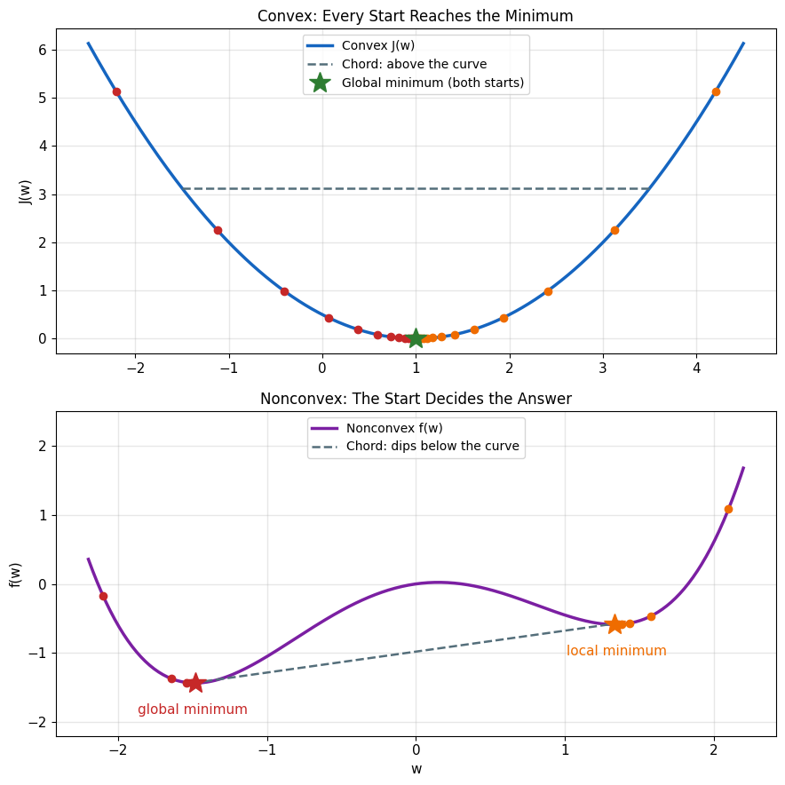
Definition: \(f\) is convex if for all \(\lambda \in [0,1]\):
\[f(\lambda \mathbf{w}_1 + (1-\lambda)\mathbf{w}_2) \leq \lambda f(\mathbf{w}_1) + (1-\lambda)f(\mathbf{w}_2)\]
Squared loss is convex:
\[J(\mathbf{w}) = \frac{1}{2n}\|\mathbf{y} - \mathbf{X}\mathbf{w}\|^2\]
Proof via Hessian:
\[\nabla^2 J = \frac{1}{n}\mathbf{X}^T\mathbf{X}\]
Since \(\mathbf{X}^T\mathbf{X} \succeq 0\) (positive semidefinite):
\[\mathbf{v}^T(\mathbf{X}^T\mathbf{X})\mathbf{v} = \|\mathbf{X}\mathbf{v}\|^2 \geq 0 \quad \forall \mathbf{v}\]
Therefore \(J\) is convex.
- Any local minimum is global minimum
- A minimizer always exists; unique if \(\mathbf{X}^T\mathbf{X} \succ 0\)
- Gradient descent converges to global minimum for a small enough step size
- No need for random restarts
Strong convexity if \(\mathbf{X}\) full column rank:
\[J(\mathbf{w}) \geq J(\mathbf{w}^*) + \frac{\mu}{2}\|\mathbf{w} - \mathbf{w}^*\|^2\]
where \(\mu = \lambda_{\min}(\mathbf{X}^T\mathbf{X})/n > 0\)
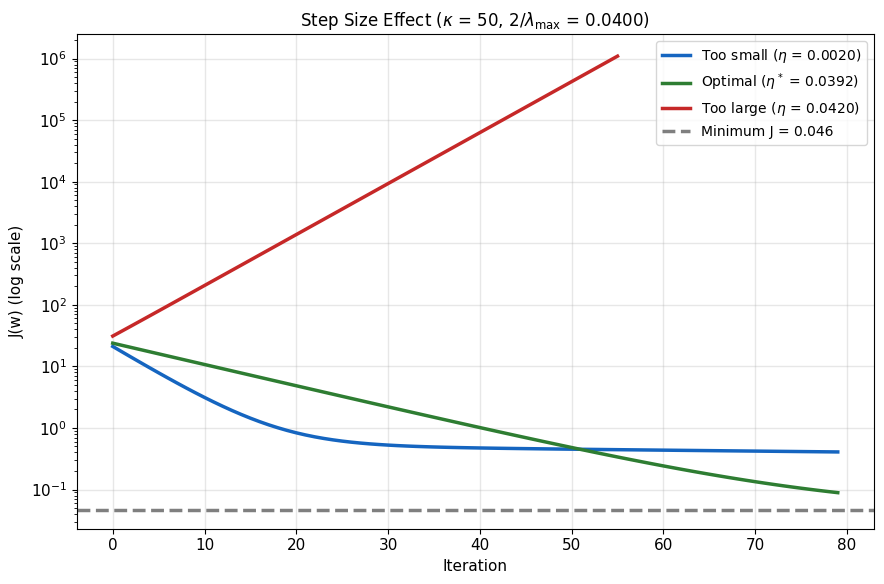
Step Size Must Stay Below \(2/\lambda_{\max}\)
Error recursion (quadratic \(J\), Hessian \(\mathbf{H} = \frac{1}{n}\mathbf{X}^T\mathbf{X}\)):
\[\mathbf{w}_{t+1} - \mathbf{w}^* = (\mathbf{I} - \eta\mathbf{H})(\mathbf{w}_t - \mathbf{w}^*)\]
- Along eigenvector \(i\) of \(\mathbf{H}\), the error scales by \(1 - \eta\lambda_i\) each step
Too small: Slow convergence
\[\mathbf{w}_{t+1} \approx \mathbf{w}_t\]
Too large: Overshoot, divergence
\[J(\mathbf{w}_{t+1}) > J(\mathbf{w}_t)\]
Theoretical bounds: need \(|1 - \eta\lambda_i| < 1\) for every \(i\):
\[0 < \eta < \frac{2}{\lambda_{\max}(\mathbf{H})}\]
Optimal step size:
\[\eta^* = \frac{2}{\lambda_{\min} + \lambda_{\max}}\]
Convergence rate (\(\kappa = \lambda_{\max}/\lambda_{\min}\)):
\[\|\mathbf{w}_t - \mathbf{w}^*\| \leq \left(\frac{\kappa - 1}{\kappa + 1}\right)^t \|\mathbf{w}_0 - \mathbf{w}^*\|\]
Condition Number Sets Convergence Speed
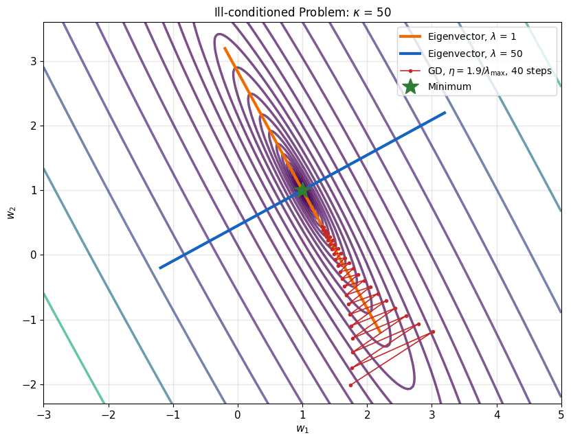
Loss surface shape: set by eigenvalues of \(\mathbf{H} = \frac{1}{n}\mathbf{X}^T\mathbf{X}\)
Principal axes: Eigenvectors of \(\mathbf{H}\)
Curvature along axis: Eigenvalue
Gradient descent behavior:
- Fast along high curvature (large \(\lambda\))
- Slow along low curvature (small \(\lambda\))
- Zigzag when \(\kappa\) is large
\(\kappa(\mathbf{H}) = \kappa(\mathbf{X})^2\): gradient descent pays for conditioning in steps, the normal equations in digits
Preconditioning: make all eigenvalues equal
\[\tilde{\mathbf{X}} = \mathbf{X}\mathbf{P}^{-1}, \quad \tilde{\mathbf{X}}^T\tilde{\mathbf{X}} = \mathbf{I}\]
- \(\mathbf{P} = \mathbf{R}\) from QR: one choice
- Feature scaling: the diagonal case
Iterations per 10× error reduction (at \(\eta^*\)):
- \(\kappa = 10\): 12
- \(\kappa = 100\): 115
- \(\kappa = 1000\): 1150
Mismatched Scales Slow Convergence
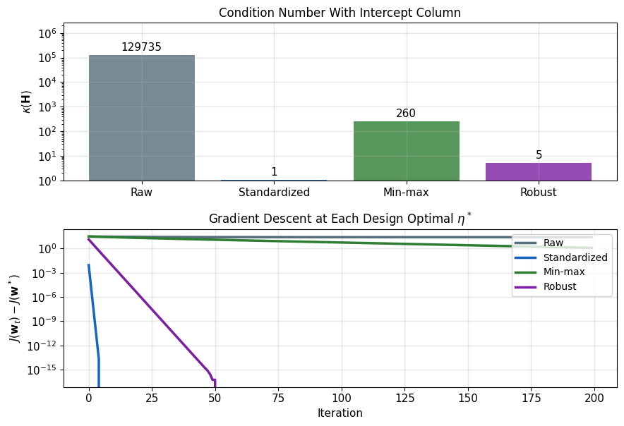
Scale mismatch inflates \(\kappa(\mathbf{H})\) (figure):
- Raw features: \(\kappa \approx 10^5\)
- Standardized: \(\kappa \approx 1\)
Rescaling:
- Changes gradient descent speed and the ridge penalty
- Leaves least-squares predictions unchanged
Standardization (z-score): \(x' = (x - \mu)/\sigma\)
- Zero mean, unit variance (the default choice)
- Preserves outliers
Min-Max scaling: \(x' = (x - x_{min})/(x_{max} - x_{min})\)
- Maps to [0, 1]
- Sensitive to outliers
- Bounded output
- Does not center: \(\kappa \approx 260\) in the figure
Robust scaling: \(x' = (x - \text{median})/\text{IQR}\)
- Uses median and interquartile range
- Robust to outliers
One Sample Gives an Unbiased Gradient
Use one sample at a time:
\[\mathbf{w}_{t+1} = \mathbf{w}_t - \eta_t \nabla \ell_{i_t}(\mathbf{w}_t)\]
where \(i_t\) randomly selected
For squared loss (\(\ell_i = \frac{1}{2}(y_i - \mathbf{w}^T\mathbf{x}_i)^2\)):
\[\nabla \ell_i(\mathbf{w}) = -(y_i - \mathbf{w}^T \mathbf{x}_i)\mathbf{x}_i\]
LMS algorithm (Widrow-Hoff) is SGD for squared loss: \(\mathbf{w}_{t+1} = \mathbf{w}_t + \eta e_t \mathbf{x}_t\)
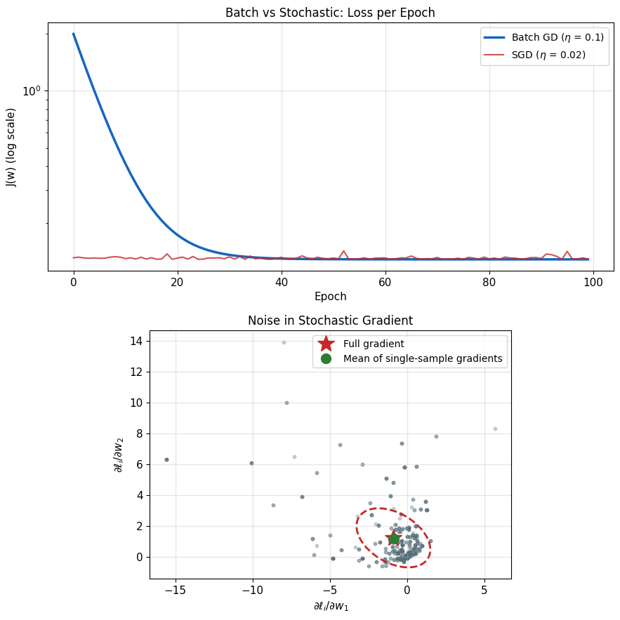
Unbiased gradient estimate:
\[\mathbb{E}[\nabla \ell_i(\mathbf{w})] = \nabla J(\mathbf{w})\]
Noise in gradient:
\[\text{Var}[\nabla \ell_i] = \mathbb{E}[\|\nabla \ell_i\|^2] - \|\nabla J\|^2\]
Cost and use:
- Cheap iteration: \(O(p)\) vs \(O(np)\)
- Online learning capability
Constant Step Size Stalls at a Noise Floor
Fixed step size: Converges to neighborhood
\[\mathbb{E}[\|\mathbf{w}_t - \mathbf{w}^*\|^2] \leq (1 - \eta\mu)^t\|\mathbf{w}_0 - \mathbf{w}^*\|^2 + O\!\left(\frac{\eta\sigma_g^2}{\mu}\right)\]
where \(\sigma_g^2\) = gradient noise variance, \(\mu = \lambda_{\min}(\mathbf{H})\)
Decreasing step size: Converges to exact solution
Required conditions (Robbins-Monro):
\[\sum_{t=1}^{\infty} \eta_t = \infty, \quad \sum_{t=1}^{\infty} \eta_t^2 < \infty\]
Example: \(\eta_t = \eta_0/t\)
Lowering the floor:
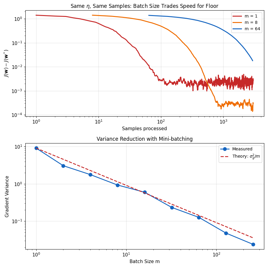
- Mini-batching: gradient variance \(\sigma_g^2/m\)
- Decreasing \(\eta_t\)
- Momentum, Adam, RMSprop change the step, not the gradient variance
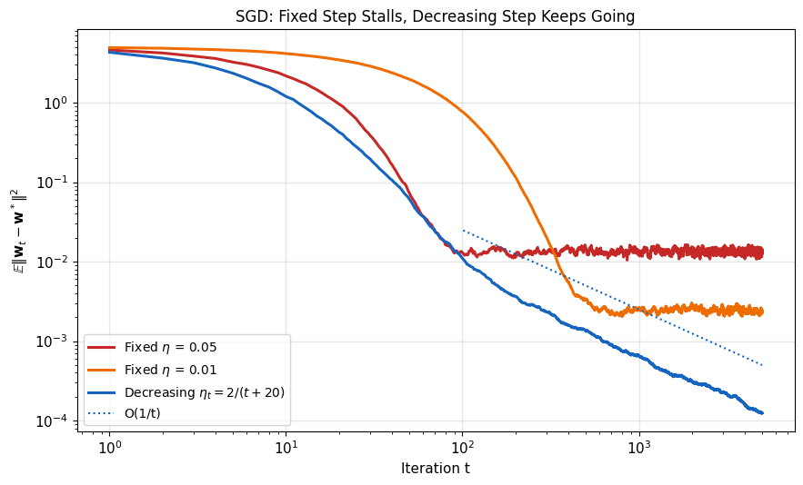
Convergence rates:
| Method | Rate | Final Error |
|---|---|---|
| Batch GD | \(\left(\frac{\kappa-1}{\kappa+1}\right)^t\) | 0 |
| SGD (fixed \(\eta\)) | \((1 - \eta\mu)^t\) | \(O(\eta)\) |
| SGD (decreasing) | \(O(1/t)\) | 0 |
Mini-batches Divide Gradient Variance by \(m\)
Mini-batch gradient:
\[\nabla J_{\mathcal{B}} = \frac{1}{m} \sum_{i \in \mathcal{B}} \nabla \ell_i(\mathbf{w})\]
where \(|\mathcal{B}| = m\) = batch size
Variance reduction:
\[\text{Var}[\nabla J_{\mathcal{B}}] = \frac{1}{m}\text{Var}[\nabla \ell_i]\]
Consequences:
- Gradient noise (std) falls by \(\sqrt{m}\)
- The noise floor \(O(\eta\sigma_g^2/(m\mu))\) allows a larger \(\eta\) at the same floor
- The \(m\) gradients compute in parallel (one pass on a GPU)
Epoch: One pass through dataset
- Batch: 1 update per epoch
- SGD: \(n\) updates per epoch
- Mini-batch: \(n/m\) updates per epoch
Equal compute:
- One step with \(m\) samples: variance \(\sigma_g^2/m\)
- \(m\) single-sample steps: same samples, \(m\) updates
- The gain from batching is parallel hardware, not fewer samples
\(\hat{\mathbf{w}}\) Is a Random Variable
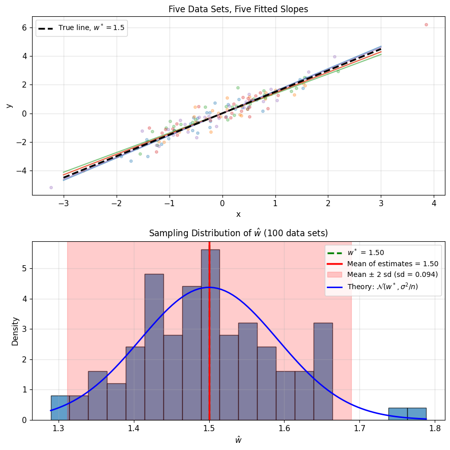
Model: \(\mathbf{y} = \mathbf{X}\mathbf{w}^* + \epsilon\), \(\;\epsilon \sim \mathcal{N}(\mathbf{0}, \sigma^2\mathbf{I})\)
Substitute into the least-squares solution:
\[\hat{\mathbf{w}} = (\mathbf{X}^T\mathbf{X})^{-1}\mathbf{X}^T\mathbf{y} = \mathbf{w}^* + (\mathbf{X}^T\mathbf{X})^{-1}\mathbf{X}^T\epsilon\]
- New noise draw, new \(\hat{\mathbf{w}}\)
- \(\mathbb{E}[\hat{\mathbf{w}}] = \mathbf{w}^*\): unbiased
Spread of \(\hat{\mathbf{w}}\): set by \(\sigma^2\), \(n\), and \(\mathbf{X}\)
Statistical inference:
- Point estimate \(\hat{\mathbf{w}}\): where
- \(\text{Cov}(\hat{\mathbf{w}})\): how sure
- Confidence region: where \(\mathbf{w}^*\) likely lies
Covariance of \(\hat{\mathbf{w}}\) Is \(\sigma^2(\mathbf{X}^T\mathbf{X})^{-1}\)
From \(\hat{\mathbf{w}} - \mathbf{w}^* = (\mathbf{X}^T\mathbf{X})^{-1}\mathbf{X}^T\epsilon\):
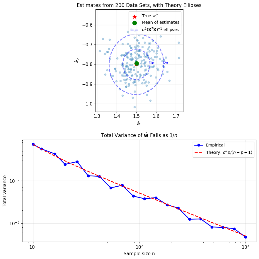
\[\text{Cov}(\hat{\mathbf{w}}) = \sigma^2(\mathbf{X}^T \mathbf{X})^{-1}\]
- Large eigenvalues of \(\mathbf{X}^T \mathbf{X}\): precise
- Small eigenvalues: uncertain along those directions
Fisher information (curvature of the log-likelihood):
\[\mathcal{I} = -\mathbb{E}\left[\nabla^2 \log L(\mathbf{w})\right] = \frac{1}{\sigma^2}\mathbf{X}^T \mathbf{X}\]
- \(\text{Cov}(\hat{\mathbf{w}}) = \mathcal{I}^{-1}\): sharper peak, smaller variance
Confidence region: the ellipsoid \((\hat{\mathbf{w}} - \mathbf{w}^*)^T \mathcal{I} (\hat{\mathbf{w}} - \mathbf{w}^*) \leq c\)
- Axes along the eigenvectors of \(\mathbf{X}^T\mathbf{X}\), longest where its eigenvalue is smallest
Cramér-Rao bound: any unbiased estimator \(\tilde{\mathbf{w}}\) has \(\text{Cov}(\tilde{\mathbf{w}}) \succeq \mathcal{I}^{-1}\)
- Least squares attains it for every \(n\)
- Lower variance requires bias
Near-Singular \(\mathbf{X}^T\mathbf{X}\) Inflates the Variance
\(\sigma^2(\mathbf{X}^T\mathbf{X})^{-1}\) grows without bound when:
- \(p > n\): singular, infinitely many solutions
- Polynomial features of degree \(k\) on \(d\) inputs: \(p = \binom{d+k}{k}\), \(\;d = 100\), \(k = 3\) gives \(p = 176{,}851\)
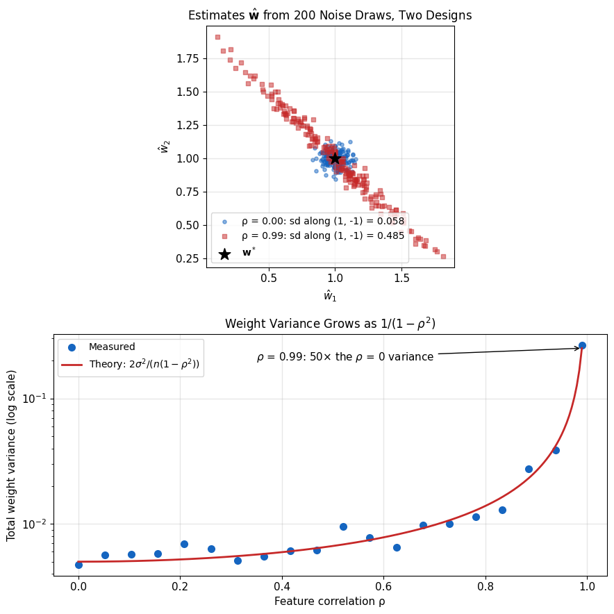
- Collinear features: nearly singular, variance \(\propto 1/(1 - \rho^2)\)
- \(\rho = 0.99\): 50× the variance of uncorrelated features
- The uncertainty lies along the eigenvector with the smallest eigenvalue (figure)
Way out: add a penalty \(R(\mathbf{w})\) on complexity, \(J(\mathbf{w}) + \lambda R(\mathbf{w})\)
- Unique solution even if \(p > n\)
- Lower variance, at the cost of bias
- \(\lambda\) controls model complexity
Prediction Error Decomposes into Bias, Variance, and Noise
Setup: \(y = f(x) + \epsilon\), \(\;\mathbb{E}[\epsilon] = 0\), \(\;\text{Var}(\epsilon) = \sigma^2\)
Expand at point \(x_0\), with \(\hat{f}\) random (trained on random data):
\[\mathbb{E}[(y - \hat{f}(x_0))^2] = \mathbb{E}[(f(x_0) + \epsilon - \hat{f}(x_0))^2]\]
Independence of \(\epsilon\) and \(\hat{f}\):
\[= \mathbb{E}[(f(x_0) - \hat{f}(x_0))^2] + \sigma^2\]
Add and subtract \(\mathbb{E}[\hat{f}(x_0)]\):
\[= \text{Var}(\hat{f}(x_0)) + (f(x_0) - \mathbb{E}[\hat{f}(x_0)])^2 + \sigma^2\]
\[\boxed{\text{MSE} = \text{Variance} + \text{Bias}^2 + \sigma^2}\]
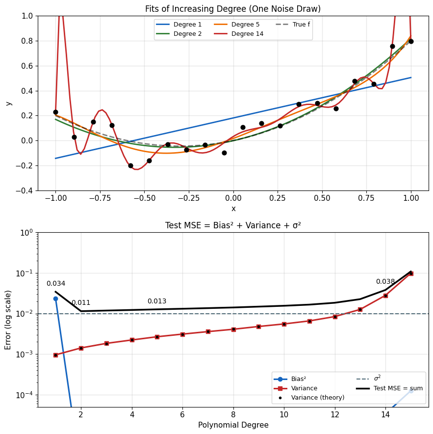
For linear models, averaged over the training inputs (what the figure measures):
- Variance: \(\frac{\sigma^2}{n}\text{tr}\left(\mathbf{X}(\mathbf{X}^T\mathbf{X})^{-1}\mathbf{X}^T\right) = p\sigma^2/n\)
- Bias decreases as \(p\) increases (nested models)
Measured (polynomial degree, \(n = 20\), \(\sigma = 0.1\), the figure’s setup):
| Degree | Bias\(^2\) | Variance | Test MSE |
|---|---|---|---|
| 1 | 0.023 | 0.001 | 0.034 |
| 2 | < 0.001 | 0.001 | 0.011 |
| 5 | < 0.001 | 0.003 | 0.013 |
| 14 | < 0.001 | 0.028 | 0.038 |
Overfitting:
- Variance dominates bias
- Training error \(\ll\) test error
L2 Penalty Guarantees a Unique, Stable Solution
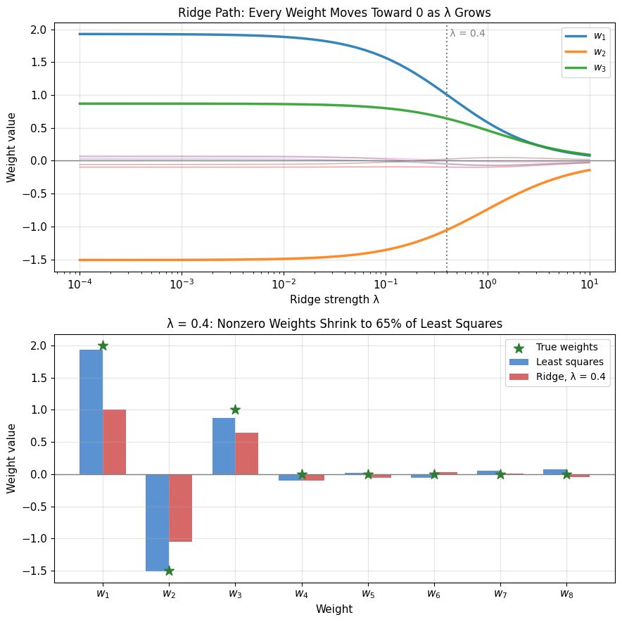
Ridge regression (L2 penalty on every weight but the intercept \(w_0\)):
\[J_\lambda(\mathbf{w}) = \frac{1}{2n}\|\mathbf{y} - \mathbf{X}\mathbf{w}\|^2 + \frac{\lambda}{2} \sum_{j \geq 1} w_j^2\]
Solution (\(\nabla J_\lambda = \mathbf{0}\)), with \(\mathbf{D} = \text{diag}(0, 1, \ldots, 1)\):
\[\hat{\mathbf{w}}_{\text{ridge}} = (\mathbf{X}^T \mathbf{X} + n\lambda \mathbf{D})^{-1} \mathbf{X}^T \mathbf{y}\]
Effect:
- Invertible for any \(\lambda > 0\), even \(p > n\)
- Shrinks weights toward zero: less variance, some bias
- Component of \(\hat{\mathbf{w}}_{\text{OLS}}\) along right singular vector \(\mathbf{v}_i\) scaled by \(\sigma_i^2/(\sigma_i^2 + n\lambda)\): small \(\sigma_i\) shrink most
- Penalty depends on feature scale: a feature in cm carries \(10^4\times\) the penalty of the same feature in m, so standardize first
Ridge Is MAP with a Gaussian Prior
Posterior: \(p(\mathbf{w}|\mathcal{D}) \propto p(\mathcal{D}|\mathbf{w}) \cdot p(\mathbf{w})\)
MAP estimation:
\[\hat{\mathbf{w}}_{\text{MAP}} = \arg\max_{\mathbf{w}} [\log p(\mathcal{D}|\mathbf{w}) + \log p(\mathbf{w})]\]
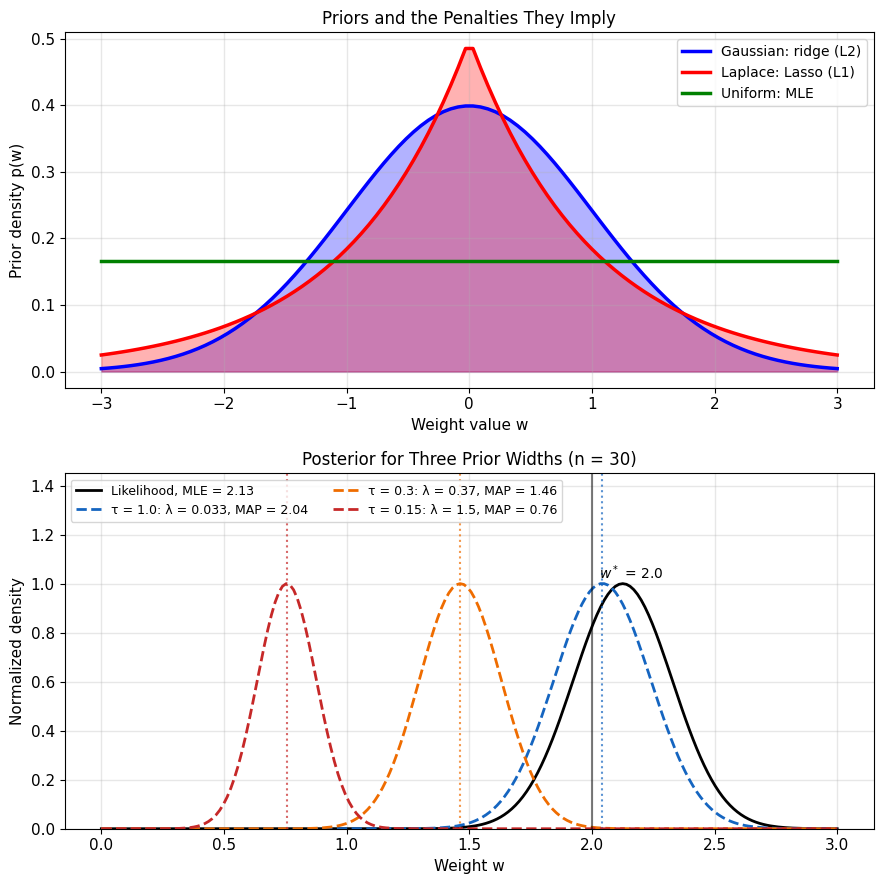
Gaussian prior \(\mathbf{w} \sim \mathcal{N}(\mathbf{0}, \tau^2 \mathbf{I})\): \(\;\log p(\mathbf{w}) = -\frac{1}{2\tau^2}\|\mathbf{w}\|^2 + \text{const}\)
\[\hat{\mathbf{w}}_{\text{MAP}} = \arg\min_{\mathbf{w}} \left[\frac{1}{2\sigma^2}\|\mathbf{y} - \mathbf{X}\mathbf{w}\|^2 + \frac{1}{2\tau^2}\|\mathbf{w}\|^2\right]\]
- Divide by \(n/\sigma^2\): ridge with \(\lambda = \sigma^2/(n\tau^2)\)
- Narrow prior (small \(\tau\)): large \(\lambda\)
- More data (large \(n\)): the prior counts for less
Other priors:
- Uniform: MAP = MLE
- Laplace prior: L1 penalty \(\lambda\|\mathbf{w}\|_1\), the Lasso (a Laplace noise model gives LAD instead)
The Test Set Is Used Once
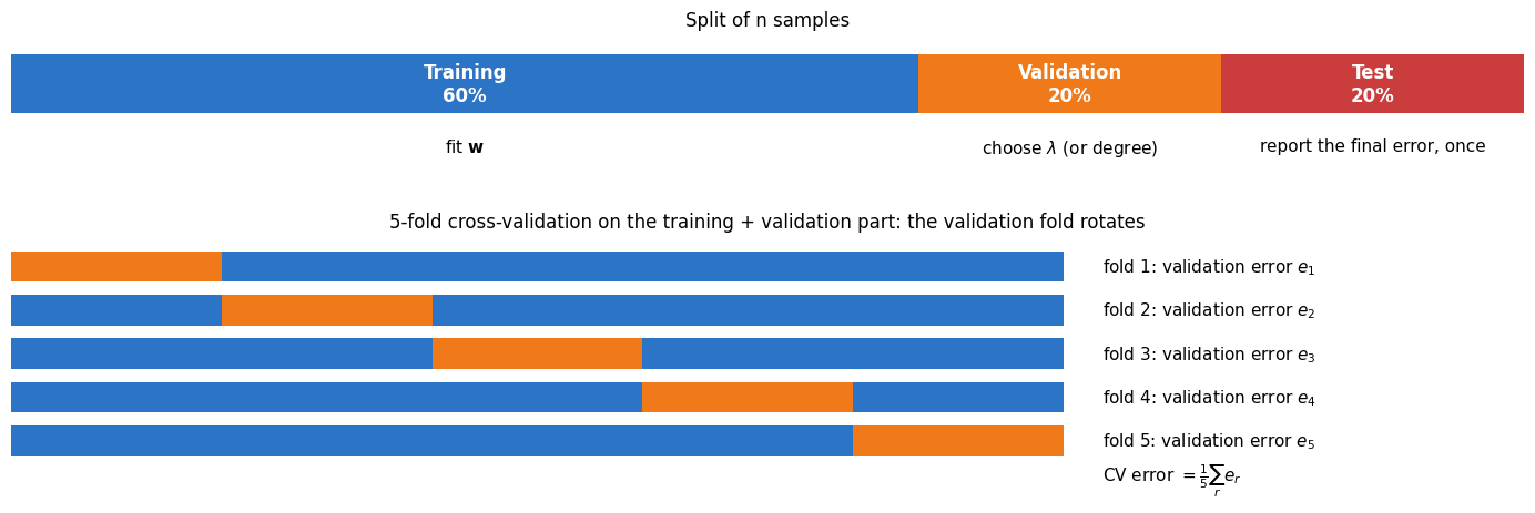
- Training error: loss on the data used to fit \(\mathbf{w}\)
- Test error: loss on held-out data, never seen during training
- Overfitting: a large gap between the two
- Cross-validation: rotate the validation fold when data are scarce, average the \(k\) errors
Validation Error Sets \(\lambda\)
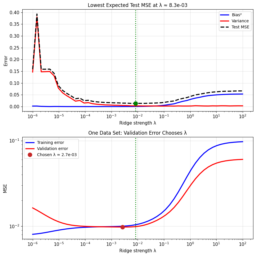
Effect of \(\lambda\):
- \(\lambda = 0\): low bias, high variance
- \(\lambda \to \infty\): \(\mathbf{w} \to \mathbf{0}\), high bias, zero variance
- Chosen \(\lambda\): minimum validation error, never the test error
In the figure:
- Top: expected test MSE over 200 training sets, its minimum in green
- Bottom: one training set, one validation set, the chosen \(\lambda\) in red, close to the green line
Rare Events Carry More Information
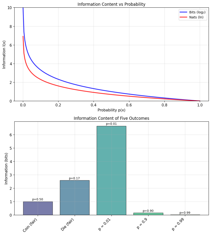
Information content of a single outcome \(x\):
\[I(x) = -\log p(x)\]
Units: bits (base 2), nats (base \(e\), used from here on)
Properties:
- \(I(x) \geq 0\)
- \(p(x) = 1 \Rightarrow I(x) = 0\): a certain event carries nothing
- \(p(x) \to 0 \Rightarrow I(x) \to \infty\)
Logarithm: information from independent events adds
\[I(A \cap B) = -\log p(A)p(B) = I(A) + I(B)\]
Fair coin: \(I(\text{heads}) = -\log_2 0.5 = 1\) bit
Entropy Is the Expected Information
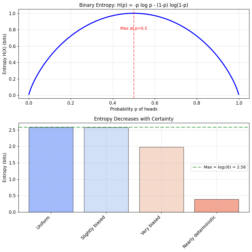
Entropy: expected information content over all outcomes
\[H(X) = \mathbb{E}[I(X)] = -\sum_x p(x) \log p(x)\]
Interpretation:
- Average uncertainty before observing \(X\)
- Average surprise when observing \(X\)
- Minimum bits to encode \(X\), on average
Properties:
- \(H(X) \geq 0\)
- \(H(X) = 0 \iff X\) is deterministic
- \(H(X) \leq \log |\mathcal{X}|\), equality for the uniform distribution on the outcome set \(\mathcal{X}\)
Examples: fair coin 1 bit, coin with \(p = 0.9\) 0.47 bits, fair die \(\log_2 6 = 2.58\) bits
Differential Entropy Can Be Negative
Continuous case: the sum becomes an integral
\[H(X) = -\int p(x) \log p(x) \, dx\]
Not bounded below:
- Uniform on \([0, \tfrac{1}{2}]\): \(H = \log \tfrac{1}{2} < 0\)
- A density can exceed 1, so \(-\log p\) can be negative
Still meaningful:
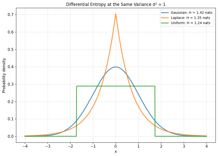
- Comparisons at a fixed constraint (figure)
- Differences, which is all the loss functions use
Gaussian: \(H = \tfrac{1}{2}\log(2\pi e \sigma^2)\), negative for \(\sigma < 0.24\)
Gaussian Has the Most Entropy at Fixed Variance
Maximum entropy principle: among all distributions meeting the known constraints, take the one with the largest entropy
- It encodes the constraints and nothing else
Known mean and variance:
\[\max_{p} H(p) \quad \text{s.t.} \quad \mathbb{E}[X] = \mu, \; \text{Var}(X) = \sigma^2\]
Solution: \(\mathcal{N}(\mu, \sigma^2)\)
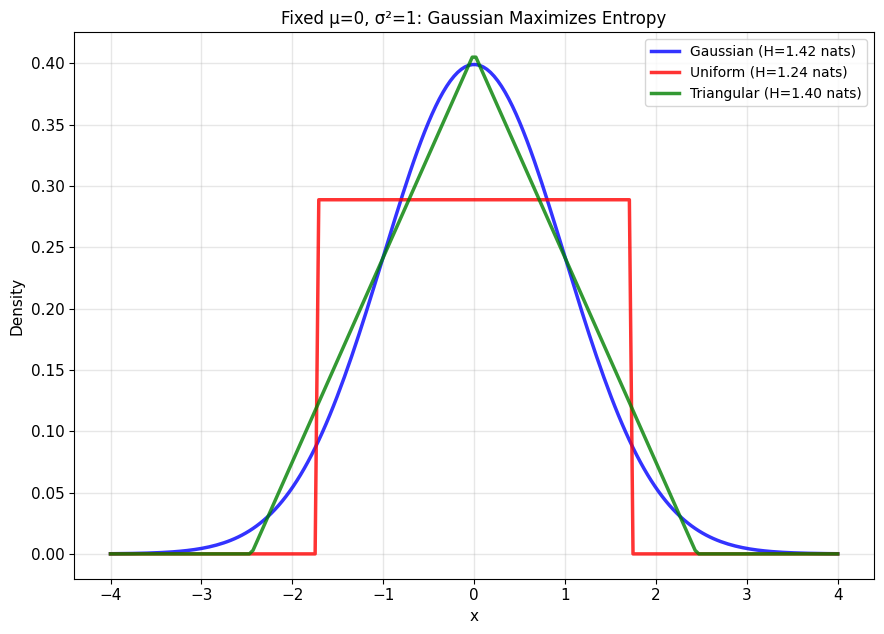
- Uniform, triangular, any other density with the same \(\mu\), \(\sigma^2\): lower entropy (figure)
Laplace Has the Most Entropy at Fixed Mean Deviation
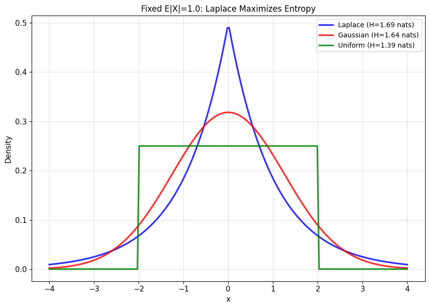
Known mean absolute deviation:
\[\max_{p} H(p) \quad \text{s.t.} \quad \mathbb{E}|X| = b\]
Solution: Laplace with scale \(b\)
- Gaussian with the same \(\mathbb{E}|X|\): lower entropy (figure)
The two noise models of MLE:
- Squared loss assumes a variance and nothing else
- Absolute loss assumes a mean deviation and nothing else
Using the Wrong Distribution Has a Cost
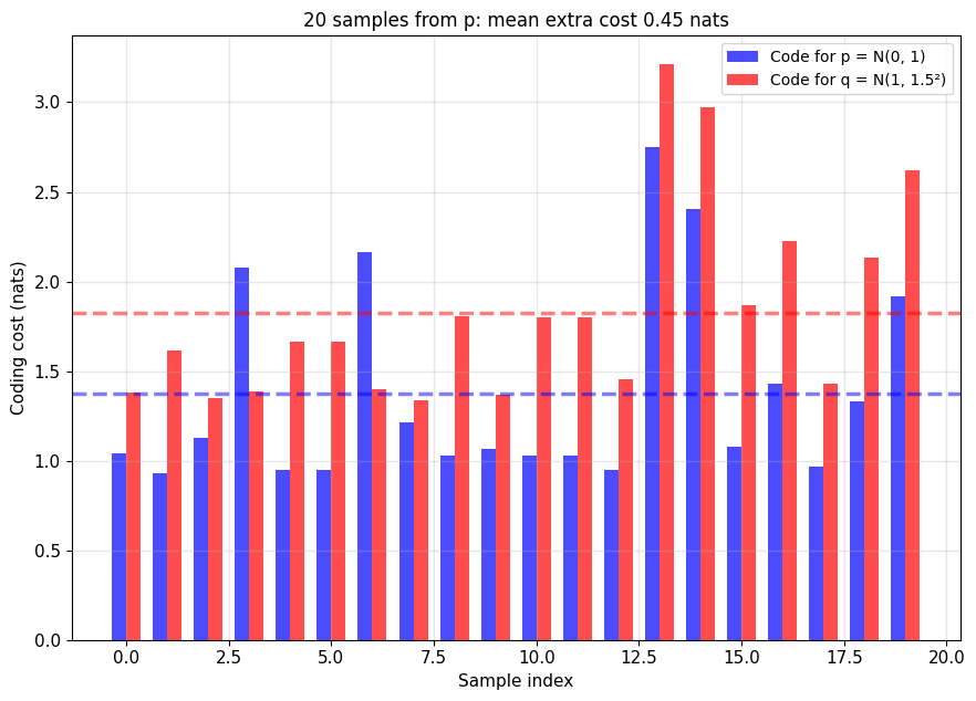
Coding: samples come from \(p\), the code was built for \(q\)
- Code length for \(x\): \(-\log q(x)\) nats
- Expected cost: \(\mathbb{E}_p[-\log q(X)]\)
Cross-entropy: the expected cost of coding \(p\) with \(q\)
\[H(p, q) = -\mathbb{E}_p[\log q(X)]\]
Cost with the right code: \(H(p, p) = H(p)\)
Extra cost: \(H(p, q) - H(p) \geq 0\), zero iff \(q = p\)
Cross-Entropy Is Entropy Plus KL Divergence
The extra cost has a name:
\[\underbrace{\mathbb{E}_p[-\log q(X)]}_{H(p,q)} - \underbrace{\mathbb{E}_p[-\log p(X)]}_{H(p)} = D_{KL}(p\|q)\]
Decomposition:
\[H(p, q) = H(p) + D_{KL}(p\|q)\]
- \(H(p)\): the cost of the data itself, fixed
- \(D_{KL}(p\|q)\): the cost of the mismatch, \(\geq 0\)
Properties of cross-entropy:
- \(H(p, q) \geq H(p)\), equality iff \(q = p\)
- Not symmetric: \(H(p, q) \neq H(q, p)\)
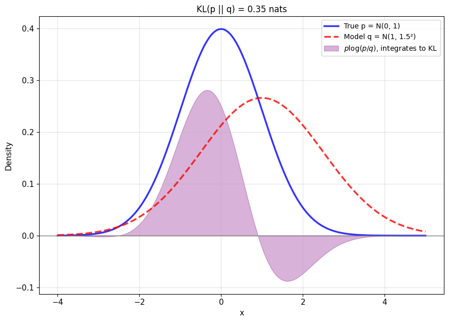
KL Divergence Is Not a Distance
Kullback-Leibler divergence:
\[D_{KL}(p\|q) = \mathbb{E}_p\left[\log \frac{p(X)}{q(X)}\right] = \int p(x) \log \frac{p(x)}{q(x)} \, dx\]
Interpretation:
- Extra nats to encode \(p\) with the code for \(q\)
- Expected log-likelihood ratio
Properties:
- \(D_{KL}(p\|q) \geq 0\): Jensen’s inequality, \(\mathbb{E}[-\log Z] \geq -\log \mathbb{E}[Z]\) for convex \(-\log\), applied to \(Z = q(X)/p(X)\) with \(\mathbb{E}_p[Z] = 1\)
- \(D_{KL}(p\|q) = 0 \iff p = q\)
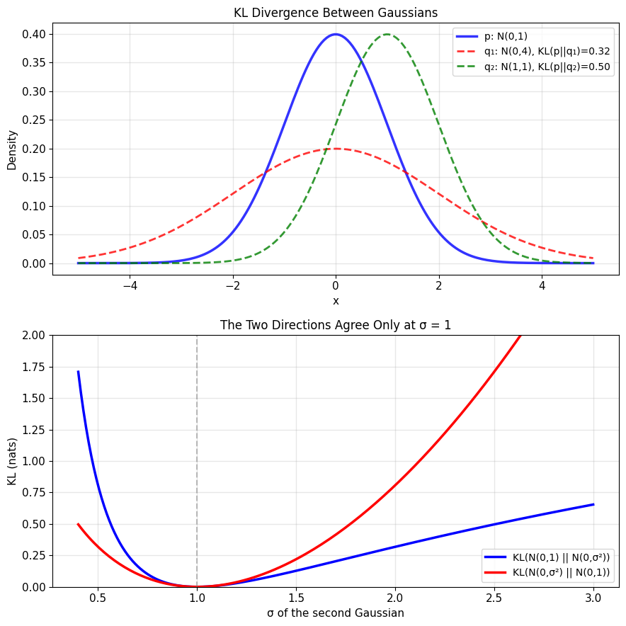
- Not symmetric: \(D_{KL}(p\|q) \neq D_{KL}(q\|p)\) (figure)
- No triangle inequality
Forward KL Covers, Reverse KL Seeks a Mode
Fit \(q\) to a fixed \(p\), two ways to score it:
Forward \(D_{KL}(p\|q) = \mathbb{E}_p[\log p/q]\):
- Weighted by \(p\)
- Wherever \(p\) has mass, \(q\) must too, or the log blows up
- Result: \(q\) spreads over every mode
Reverse \(D_{KL}(q\|p) = \mathbb{E}_q[\log q/p]\):
- Weighted by \(q\)
- Where \(q\) is zero, \(p\) is not checked
- Result: \(q\) may sit on one mode and ignore the rest
Maximum likelihood uses the forward direction
Mutual Information Is a KL Divergence
Mutual information: KL from the joint to the product of marginals
\[I(X; Y) = D_{KL}\big(p(x,y) \,\|\, p(x)p(y)\big)\]
\[= \mathbb{E}_{X,Y}\left[\log \frac{p(X,Y)}{p(X)p(Y)}\right]\]
Conditional entropy: \(H(X|Y) = -\mathbb{E}[\log p(X|Y)]\), the uncertainty left in \(X\) once \(Y\) is known
Equivalent forms:
\[I(X; Y) = H(X) - H(X|Y) = H(Y) - H(Y|X)\]
Properties:
- \(I(X; Y) \geq 0\)
- \(I(X; Y) = 0 \iff X \perp Y\)
- \(I(X; Y) = I(Y; X)\)
- \(I(X; X) = H(X)\)
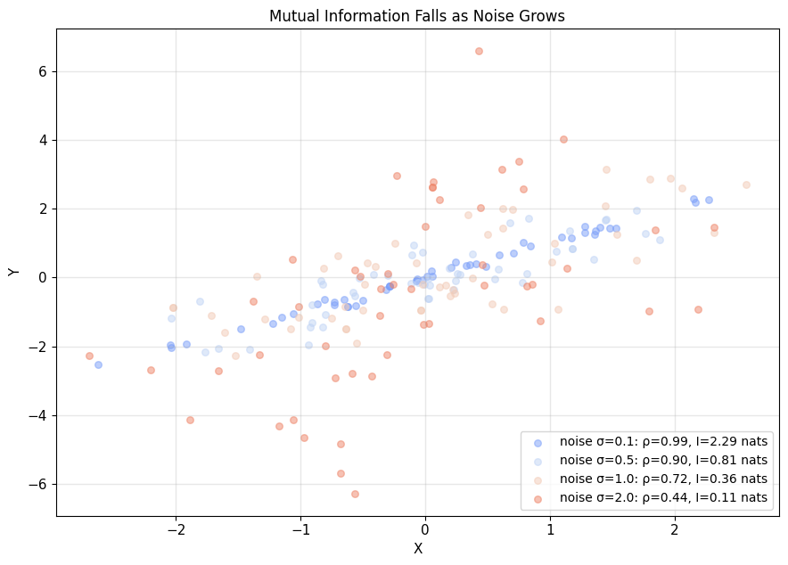
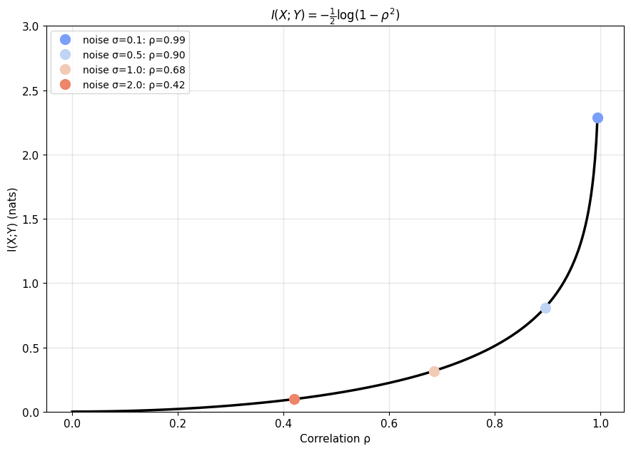
Gaussian Mutual Information Is \(-\tfrac{1}{2}\log(1 - \rho^2)\)
Bivariate Gaussian with correlation \(\rho\):
\[I(X; Y) = -\tfrac{1}{2}\log(1 - \rho^2)\]
- \(\rho = 0\): 0 nats
- \(\rho = 0.7\): 0.34 nats
- \(\rho \to 1\): unbounded
The same \(1 - \rho^2\) as the LMMSE error \(\text{Var}(Y)(1 - \rho^2)\): what the line cannot predict is what \(X\) does not tell
Data processing inequality: for a Markov chain \(X \to Y \to Z\) (\(Z\) depends on \(X\) only through \(Y\))
\[I(X; Z) \leq I(X; Y)\]
- Processing \(Y\) cannot add information about \(X\)
Maximum Likelihood Minimizes Forward KL
Setup: data from \(p\), model family \(\{q_\theta\}\)
Minimize the forward KL:
\[D_{KL}(p \,\|\, q_\theta) = -H(p) - \mathbb{E}_p[\log q_\theta(X)]\]
- \(H(p)\) does not depend on \(\theta\)
\[\arg\min_\theta D_{KL}(p \,\|\, q_\theta) = \arg\max_\theta \mathbb{E}_p[\log q_\theta(X)]\]
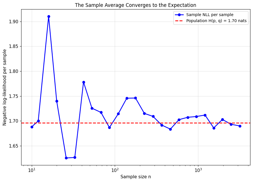
Expectation to sample average (the ERM step):
\[\mathbb{E}_p[\log q_\theta(X)] \approx \frac{1}{n}\sum_{i=1}^n \log q_\theta(x_i) = \frac{1}{n}\log L(\theta)\]
Result: maximum likelihood = ERM with \(\ell = -\log q_\theta\) = minimum forward KL
Misspecified MLE Is the Forward-KL Projection
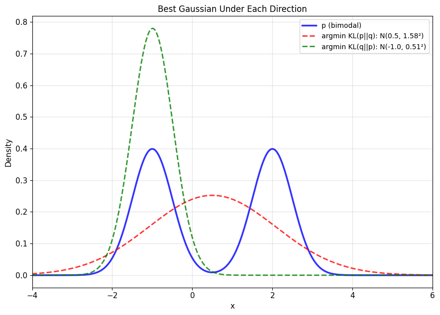
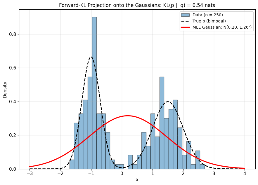
If \(p \notin \{q_\theta\}\), no \(\theta\) makes the KL zero
The minimizer: the member of the family closest to \(p\) in forward KL
- Forward direction: the fit must cover every mode
- Bimodal \(p\), Gaussian family: one wide Gaussian between the modes (figure)
What the fit gets right: the mean and variance of \(p\), exactly
What it cannot: the two modes; the KL that remains is the price of the family
Binary Labels Give Binary Cross-Entropy
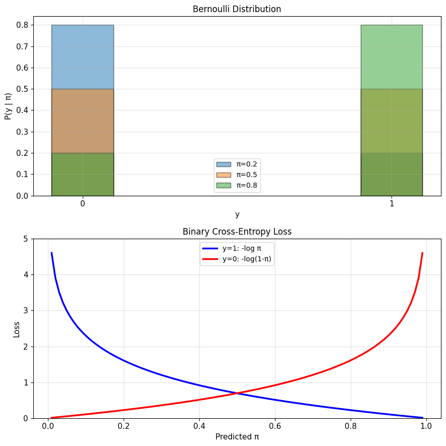
Bernoulli (\(K = 2\)): \(P(Y = 1 \,|\, \mathbf{x}) = \pi\)
\[p(y \,|\, \mathbf{x}) = \pi^y (1 - \pi)^{1-y}\]
Negative log-likelihood:
\[\ell = -y\log \pi - (1-y)\log(1-\pi)\]
Per label:
- \(y = 1\): \(-\log \pi\), zero at \(\pi = 1\)
- \(y = 0\): \(-\log(1 - \pi)\), zero at \(\pi = 0\)
Unbounded: \(\pi \to 0\) with \(y = 1\) costs without limit, a confident wrong answer is never cheap
Requires \(\pi \in (0, 1)\)
A Linear Model Cannot Output a Probability
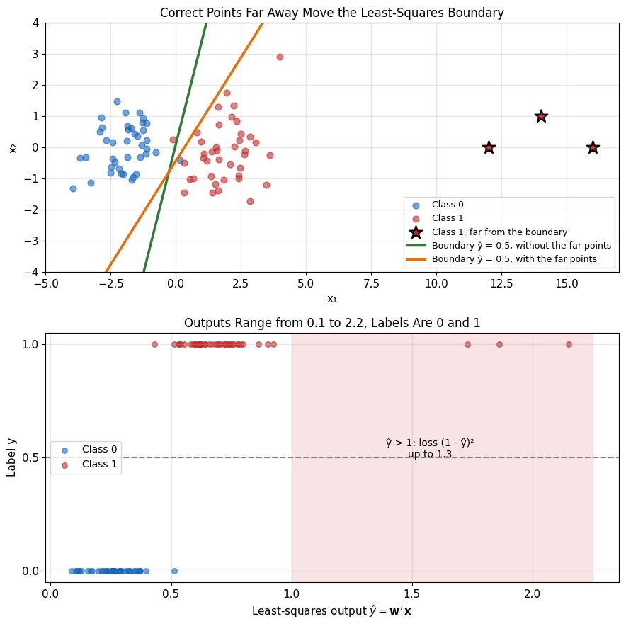
Binary labels \(y \in \{0, 1\}\) as regression: \(\hat{y} = \mathbf{w}^T\mathbf{x}\), predict 1 if \(\hat{y} > 0.5\)
- Target \(\mathbb{E}[Y \,|\, \mathbf{x}] = P(Y = 1 \,|\, \mathbf{x})\) is a probability; the model is not
Wrong class:
- \(\hat{y}\) ranges over \(\mathbb{R}\): \(\hat{y} = 2.7\) is not a probability
- Squared loss on a correct answer: \(\hat{y} = 0.9\) costs 0.01, \(\hat{y} = 5\) costs 16
- Correct points far from the boundary pull it (figure)
Wrong likelihood:
- \(Y\) is Bernoulli: variance \(\pi(1 - \pi)\), not a constant \(\sigma^2\)
- Its loss is binary cross-entropy, which needs \(\pi(\mathbf{x}) \in (0, 1)\)
Needed: a map from \(\hat{y} \in \mathbb{R}\) to \(\pi \in (0, 1)\), and the Bernoulli loss on \(\pi\)
Squashing the Linear Output Gives a Probability
Keep the linear model, add one map:
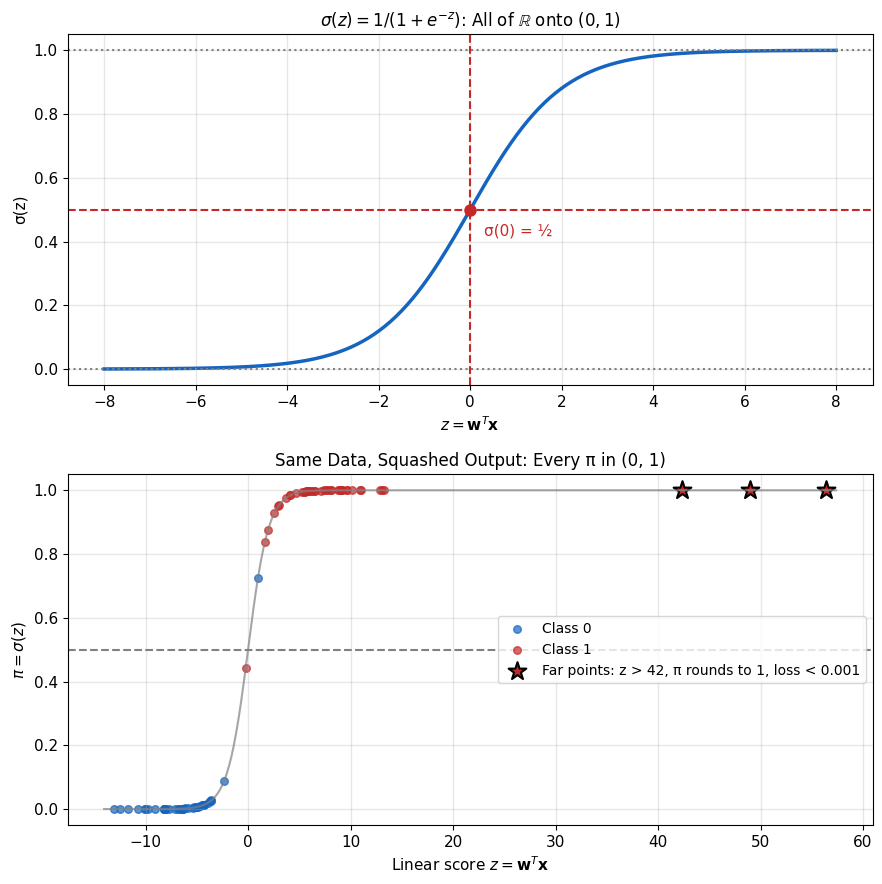
\[z = \mathbf{w}^T\mathbf{x} \in \mathbb{R} \qquad \pi = \sigma(z) = \frac{1}{1 + e^{-z}} \in (0, 1)\]
Sigmoid:
- \(\sigma(0) = \tfrac{1}{2}\): the boundary \(\mathbf{w}^T\mathbf{x} = 0\) is where \(\pi = \tfrac{1}{2}\)
- \(z \to \pm\infty\): \(\pi \to 1\) or \(0\), never reached
- \(\log \frac{\pi}{1 - \pi} = z\): the linear output is the log-odds
Model: \(P(Y = 1 \,|\, \mathbf{x}) = \sigma(\mathbf{w}^T\mathbf{x})\)
Loss: the Bernoulli negative log-likelihood
\[\ell = -y \log \sigma(z) - (1 - y)\log(1 - \sigma(z))\]
Gradient per sample: \((\sigma(z) - y)\,\mathbf{x}\), the least-squares form \((\hat{y} - y)\,\mathbf{x}\) with \(\hat{y}\) squashed