Sensors Measure with Noise
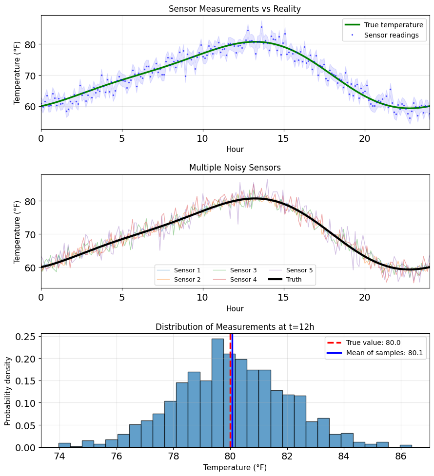
Real systems operate with incomplete information:
- Temperature sensor reads \(72^\circ\text{F} \pm 2^\circ\text{F}\)
- Radar measures distance with noise
- Stock price reflects unknown future earnings
- MRI image contains artifacts
Objective: Given measurements (\(X\)), estimate unknowns (\(Y\))
Uncertainty is inherent, not a nuisance
- Measurement noise
- Model uncertainty
- Finite samples
- Quantization effects
Many estimates of \(Y\) are possible - best needs a definition
A Predictor Is a Function of the Observation
Problem:
- \(Y\): quantity of interest (unknown)
- \(X\): observation (known)
- \((X, Y)\): jointly distributed random variables
Predictor function: \(g: \mathbb{R} \to \mathbb{R}\)
\[\hat{Y} = g(X)\]
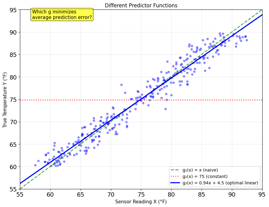
Example: Room temperature estimation
- \(Y\): true temperature
- \(X\): sensor reading = \(Y + N\)
- \(N\): measurement noise
- \(g(X) =\) ? Best guess for \(Y\) given reading \(X\)
Among all possible functions \(g\), which one is “best”?
Need:
- What we mean by “best” (loss function)
- How to deal with randomness (averaging)
The Loss Function Determines the Optimal Predictor
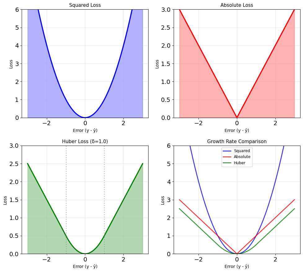
Loss function \(\ell(y, \hat{y})\) measures prediction quality
Common choices:
| Loss | Formula | Properties |
|---|---|---|
| Squared | \((y - \hat{y})^2\) | Differentiable, convex, emphasizes large errors |
| Absolute | \(|y - \hat{y}|\) | Robust to outliers, non-differentiable at 0 |
| 0-1 | \(\mathbb{1}[y \neq \hat{y}]\) | Classification, discontinuous |
| Huber | \(\begin{cases} \frac{1}{2}(y-\hat{y})^2 & |y-\hat{y}| \leq \delta \\ \delta|y-\hat{y}| - \frac{\delta^2}{2} & \text{otherwise} \end{cases}\) | Robust + differentiable |
Risk: Expected loss over joint distribution
\[R(g) = \mathbb{E}[\ell(Y, g(X))] = \int\int \ell(y, g(x)) p(x,y) \, dx \, dy\]
Goal: Find \(g^* = \arg\min_g R(g)\)
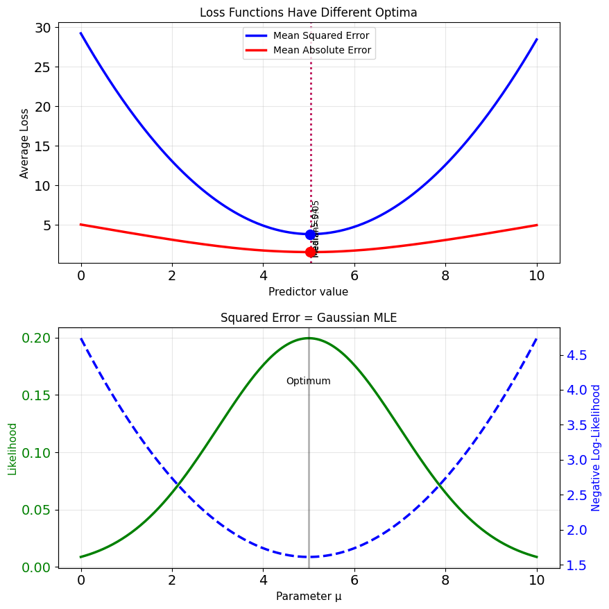
Squared error leads to the expected value (mean), absolute error the median
Squared Error Loss Gives Closed Forms
Mathematical advantages:
-
Differentiable:
\[\frac{d}{d\hat{y}}(y - \hat{y})^2 = -2(y - \hat{y})\]Smooth objective
-
Unique minimum: Strictly convex \(\Rightarrow\) no local minima
-
Closed-form solutions: Often analytically tractable
-
Decomposition:
\[\text{MSE} = \text{Bias}^2 + \text{Variance}\]Separates systematic error from random scatter
Statistical connection:
Under Gaussian noise \(N \sim \mathcal{N}(0, \sigma^2)\):
\[Y = \mu + N\]
Maximum likelihood estimation:
\[\hat{\mu}_{\text{MLE}} = \arg\max_\mu p(y|\mu) = \arg\min_\mu (y - \mu)^2\]
MSE \(\leftrightarrow\) Gaussian MLE
MSE Is the Expected Squared Error
Definition: for estimator \(g\)
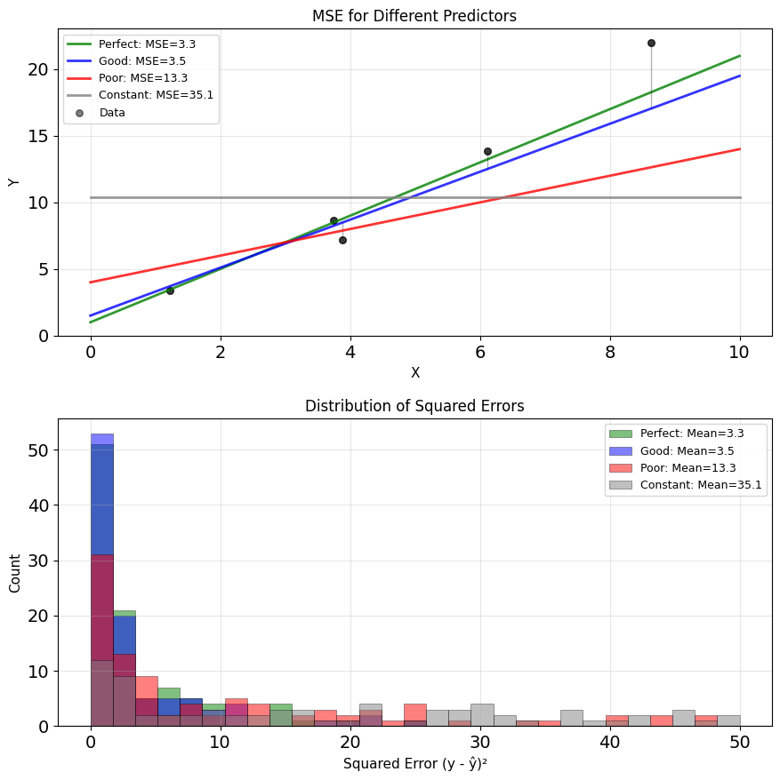
\[\text{MSE}(g) = \mathbb{E}[(Y - g(X))^2]\]
Expanding the expectation:
\[\text{MSE}(g) = \int\int (y - g(x))^2 p(x,y) \, dx \, dy\]
Empirical MSE (from data):
\[\widehat{\text{MSE}} = \frac{1}{n} \sum_{i=1}^n (y_i - g(x_i))^2\]
Properties:
- Always non-negative: \(\text{MSE} \geq 0\)
- Zero iff perfect prediction: \(\text{MSE} = 0 \iff P(Y = g(X)) = 1\)
- Units: \([\text{MSE}] = [Y]^2\)
Other forms:
- RMSE = \(\sqrt{\text{MSE}}\) (same units as \(Y\))
- Normalized MSE = MSE/Var(Y)
More Flexible Estimator = More to Know
Hierarchy of function classes:
-
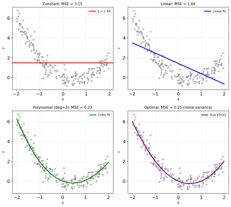
Constant: \(\hat{Y} = c\)
- Ignores observation X
- Optimal: \(c^* = \mathbb{E}[Y]\)
- MSE = Var(Y)
-
Linear (affine): \(\hat{Y} = aX + b\)
- Two parameters
- Needs only first and second moments
-
Polynomial: \(\hat{Y} = \sum_{k=0}^p a_k X^k\)
- Needs moments up to order \(2p\)
- Overfitting risk
-
Unrestricted: \(\hat{Y} = g(X)\)
- Any measurable function
- Needs the full conditional \(p(y|x)\)
Each step up fits more but requires knowing more
Linear Means Linear in \(X\)
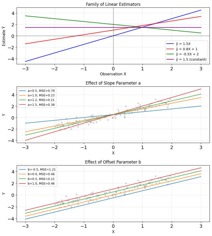
Definition: A linear estimator has the form
\[\hat{Y} = aX + b\]
where \(a, b \in \mathbb{R}\) are constants.
- \(\hat{Y} = 3X + 2\): linear in \(X\)
- \(\hat{Y} = \beta X^2\): not linear - quadratic in \(X\), though linear in \(\beta\)
Parameters:
- \(a\): slope/gain/sensitivity
- \(b\): offset/bias/intercept
Special cases:
- \(b = 0\): Proportional estimator \(\hat{Y} = aX\)
- \(a = 0\): Constant estimator \(\hat{Y} = b\)
- \(a = 1, b = 0\): Direct use \(\hat{Y} = X\)
Affine, strictly: superposition holds only for \(b = 0\)
Vector case: \(\hat{\mathbf{y}} = \mathbf{A}\mathbf{x} + \mathbf{b}\)
Means and Covariances Determine the Best Line
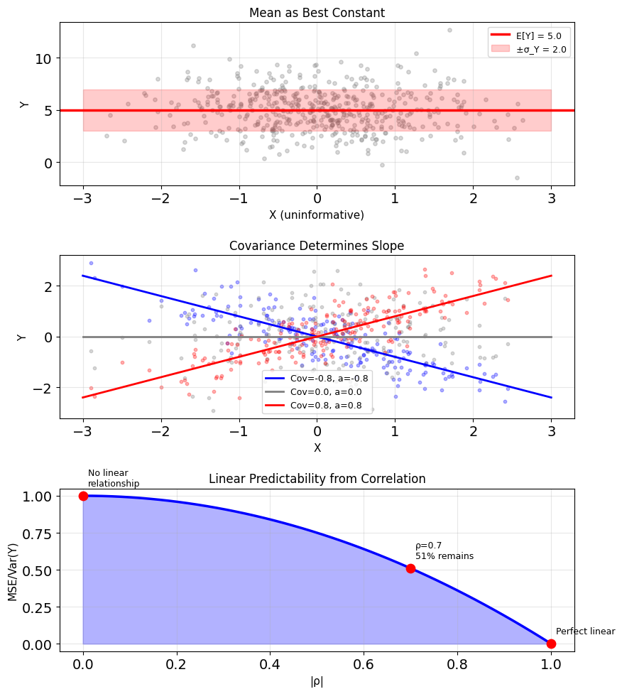
Mean \(\mathbb{E}[Y]\): baseline prediction
- Best constant; what to predict without observing \(X\)
Variance \(\text{Var}(Y)\): the error to beat
- MSE of the baseline; total variation to explain
Covariance \(\text{Cov}(X,Y)\): linear link
- Sign sets the slope direction. If zero - no linear relationship improves
Correlation \(\rho \in [-1, 1]\): scale-free link
- \(|\rho| = 1\): exact linear dependence
- \(\rho^2\) = fraction of Var(Y) a line removes
These moments completely determine the optimal linear estimator
SNR Bounds Linear Estimation Error
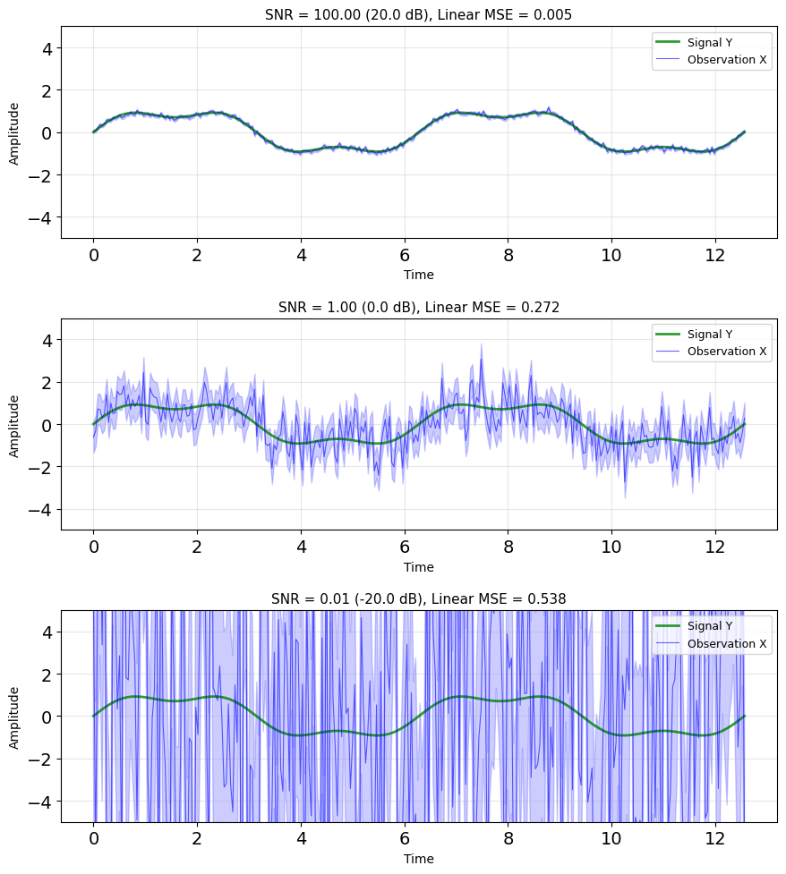
Additive noise model:
\[X = Y + N\]
- \(Y\): true signal (what we want)
- \(N\): noise (corruption)
- \(X\): observation (what we get)
- Independence: \(Y \perp N\)
Signal-to-Noise Ratio (SNR):
\[\text{SNR} = \frac{\text{Power}(Y)}{\text{Power}(N)} = \frac{\mathbb{E}[Y^2]}{\mathbb{E}[N^2]}\]
For zero-mean:
\[\text{SNR} = \frac{\sigma_Y^2}{\sigma_N^2}\]
In dB: \(\text{SNR}_{\text{dB}} = 10\log_{10}(\text{SNR})\)
Linear estimation floor:
\[\text{MSE}_{\text{L}} = \frac{\sigma_Y^2 \sigma_N^2}{\sigma_Y^2 + \sigma_N^2} = \frac{\sigma_Y^2}{1 + \text{SNR}}\]
- Residual error at every finite SNR
- Equals the overall optimum for Gaussian \(Y, N\); lower is possible otherwise
Random Variables Map Outcomes to Numbers
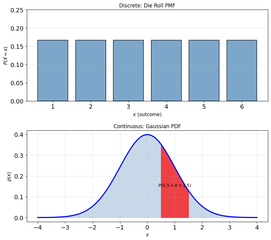
Sample space \(\Omega\): Set of all possible outcomes
Random variable \(X: \Omega \to \mathbb{R}\)
Maps each outcome to a real number.
Notation convention:
- \(X\) (uppercase): The random variable (a function)
- \(x\) (lowercase): A specific realized value
Discrete example: Die roll
- \(\Omega = \{\omega_1, \omega_2, \omega_3, \omega_4, \omega_5, \omega_6\}\)
- \(X(\omega_i) = i\)
- \(P(X = 3) = 1/6\)
Continuous example: Measurement noise
- \(\Omega\) = all possible noise realizations
- \(X(\omega)\) = voltage at time \(t\)
- \(P(X = 1.5)\) = 0, but \(P(1.4 < X < 1.6) > 0\)
The Joint Distribution is Complete
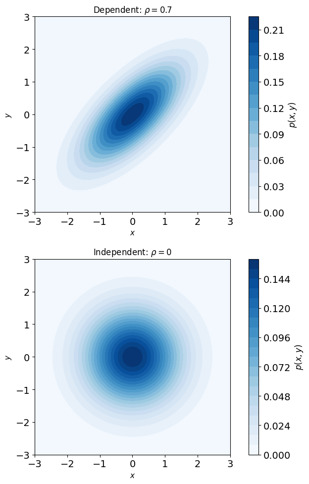
Joint distribution \(p(x, y)\):
Probability (density) that \(X = x\) AND \(Y = y\) simultaneously.
For discrete: \(P(X = x, Y = y)\)
For continuous: \(p(x,y)\) where
\[P(a < X < b, c < Y < d) = \int_a^b \int_c^d p(x,y) \, dy \, dx\]
What the joint determines:
- How likely are specific \((x, y)\) pairs?
- Are \(X\) and \(Y\) related or independent?
- Everything about marginals and conditionals
Independence means:
\[p(x, y) = p(x) \cdot p(y)\]
Joint factors into product of marginals.
Marginals and Conditionals Come From the Joint
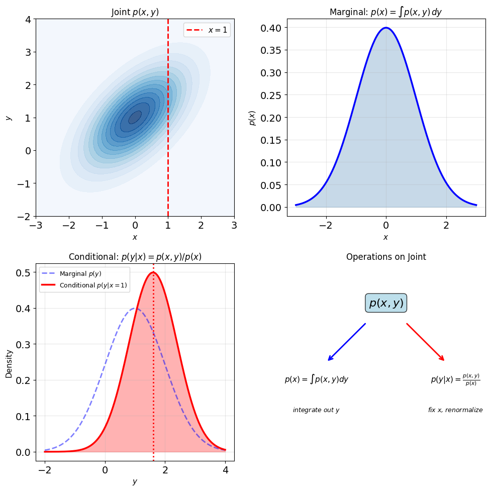
Marginal distribution: Integrate out the unused variable
\[p(x) = \int p(x, y) \, dy\]
\[p(y) = \int p(x, y) \, dx\]
Conditional distribution: Slice and renormalize
\[p(y|x) = \frac{p(x, y)}{p(x)}\]
Bayes’ rule is just rearranging:
\[p(y|x) = \frac{p(x|y) \, p(y)}{p(x)}\]
Conditioning is just:
- Start with joint \(p(x,y)\)
- Fix \(x\) to get a slice
- Divide by \(p(x)\) to make it integrate to 1
Expectation Is a Weighted Average
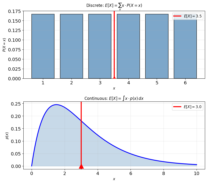
Discrete:
\[\mathbb{E}[X] = \sum_x x \cdot P(X = x)\]
Continuous:
\[\mathbb{E}[X] = \int x \cdot p(x) \, dx\]
Interpretation: Center of mass of the distribution
Expectation of a function:
\[\mathbb{E}[g(X)] = \int g(x) \cdot p(x) \, dx\]
Example: Die roll
\(\mathbb{E}[X] = 1 \cdot \frac{1}{6} + 2 \cdot \frac{1}{6} + \cdots + 6 \cdot \frac{1}{6} = 3.5\)
3.5 is not a possible outcome - it is the long-run average
Expectation Is Linear Even Under Dependence
Linearity:
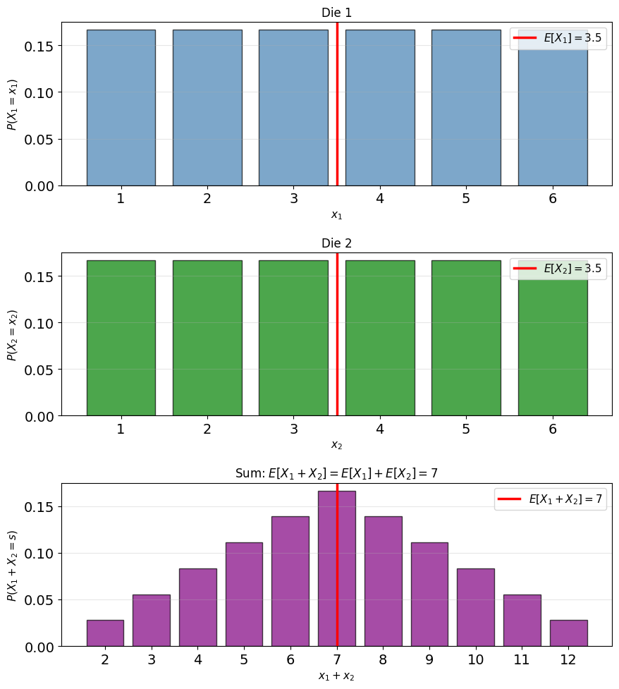
\[\mathbb{E}[aX + bY] = a\mathbb{E}[X] + b\mathbb{E}[Y]\]
This holds even if \(X\) and \(Y\) are dependent.
Why? Just rearranging sums/integrals:
\[\mathbb{E}[X + Y] = \int\int (x + y) p(x,y) \, dx \, dy\]
\[= \int\int x \, p(x,y) \, dx \, dy + \int\int y \, p(x,y) \, dx \, dy\]
\[= \int x \, p(x) \, dx + \int y \, p(y) \, dy\]
\[= \mathbb{E}[X] + \mathbb{E}[Y]\]
Example: Sum of two dice
\(\mathbb{E}[X_1 + X_2] = \mathbb{E}[X_1] + \mathbb{E}[X_2] = 3.5 + 3.5 = 7\)
i.e., Don’t need to enumerate all 36 outcomes.
Variance Measures Spread Around the Mean
Definition:
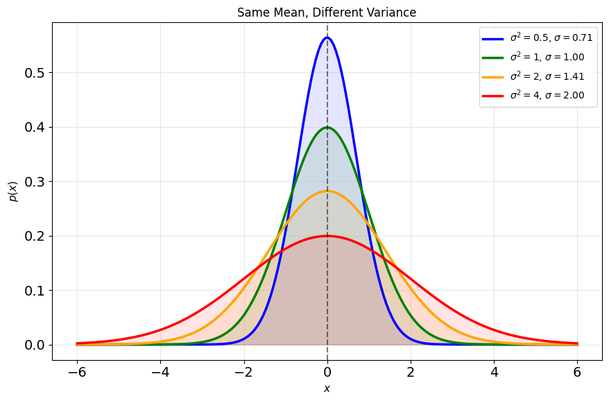
\[\text{Var}(X) = \mathbb{E}[(X - \mu)^2]\]
where \(\mu = \mathbb{E}[X]\)
Equivalent form:
\[\text{Var}(X) = \mathbb{E}[X^2] - (\mathbb{E}[X])^2\]
When to use which:
- Definition: Intuition (average squared deviation from mean)
- Equivalent form: Calculation (often simpler)
Standard deviation: \(\sigma = \sqrt{\text{Var}(X)}\)
Same units as \(X\) (variance has squared units)
Properties:
- \(\text{Var}(X) \geq 0\)
- \(\text{Var}(aX + b) = a^2 \text{Var}(X)\)
- Adding a constant shifts the mean, not the spread
Covariance Measures Linear Dependence
Definition:
\[\text{Cov}(X, Y) = \mathbb{E}[(X - \mu_X)(Y - \mu_Y)]\]
Equivalent form:
\[\text{Cov}(X, Y) = \mathbb{E}[XY] - \mathbb{E}[X]\mathbb{E}[Y]\]
Interpretation:
- \(\text{Cov} > 0\): When \(X\) is above its mean, \(Y\) tends (on average) to be above its mean
- \(\text{Cov} < 0\): When \(X\) is above its mean, \(Y\) tends to be below its mean
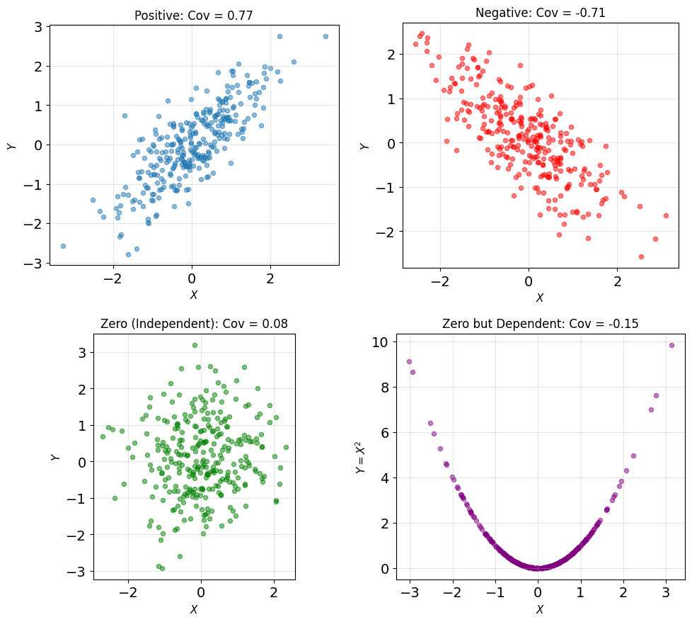
- \(\text{Cov} = 0\): No linear relationship
Correlation (normalized covariance):
\[\rho = \frac{\text{Cov}(X,Y)}{\sigma_X \sigma_Y} \in [-1, 1]\]
\(\text{Cov}(X,Y) = 0\) does NOT imply independence.
\(X \sim \mathcal{N}(0,1)\) with \(Y = X^2\): clearly dependent, but \(\text{Cov}(X, Y) = 0\).
Exception: jointly Gaussian \((X,Y)\) - zero covariance implies independence
Variance of Sums Depends on Covariance
For two random variables:
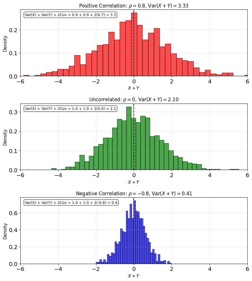
\[\text{Var}(X + Y) = \text{Var}(X) + \text{Var}(Y) + 2\text{Cov}(X, Y)\]
If uncorrelated (\(\text{Cov}(X,Y) = 0\)):
\[\text{Var}(X + Y) = \text{Var}(X) + \text{Var}(Y)\]
Compare with (linear) expectation:
- \(\mathbb{E}[X + Y] = \mathbb{E}[X] + \mathbb{E}[Y]\) always
- \(\text{Var}(X + Y) = \text{Var}(X) + \text{Var}(Y)\) only if uncorrelated
General form:
\[\text{Var}\left(\sum_i a_i X_i\right) = \sum_i a_i^2 \text{Var}(X_i) + 2\sum_{i < j} a_i a_j \text{Cov}(X_i, X_j)\]
Appears in portfolio diversification, error propagation, averaged measurements
Observations Shrink the Distribution
Joint distribution \((X, Y) \sim p(x,y)\) contains all information.
Bayes’ rule:
\[p(y|x) = \frac{p(x,y)}{p(x)} = \frac{p(x,y)}{\int p(x,y') dy'}\]
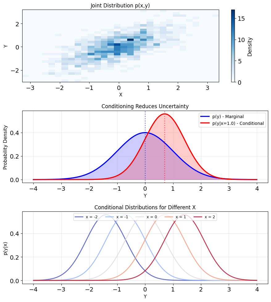
Once we observe \(X = x\), the distribution of \(Y\) changes from \(p(y)\) to \(p(y|x)\).
Example: Temperature sensor, \(X = Y + N\)
- Prior: \(Y \sim \mathcal{N}(70, 10^2)\); noise \(N \sim \mathcal{N}(0, 5^2)\)
- Observe: \(X = 75\) (sensor reading)
- Posterior: \(Y|X{=}75 \sim \mathcal{N}(74, 4.5^2)\)
Conditioning reduces uncertainty on average: \(\mathbb{E}[\text{Var}(Y|X)] \leq \text{Var}(Y)\) - a particular observation can widen the spread
Discrete case:
\[P(Y = y|X = x) = \frac{P(X = x, Y = y)}{P(X = x)}\]
\(\mathbb{E}[Y|X{=}x]\) Is a Number, \(\mathbb{E}[Y|X]\) a Random Variable
Definition: The conditional expectation of \(Y\) given \(X = x\) is:
Discrete case:
\[\mathbb{E}[Y|X=x] = \sum_y y \cdot P(Y=y|X=x)\]
Continuous case:
\[\mathbb{E}[Y|X=x] = \int_{-\infty}^{\infty} y \cdot p(y|x) \, dy\]
Facts:
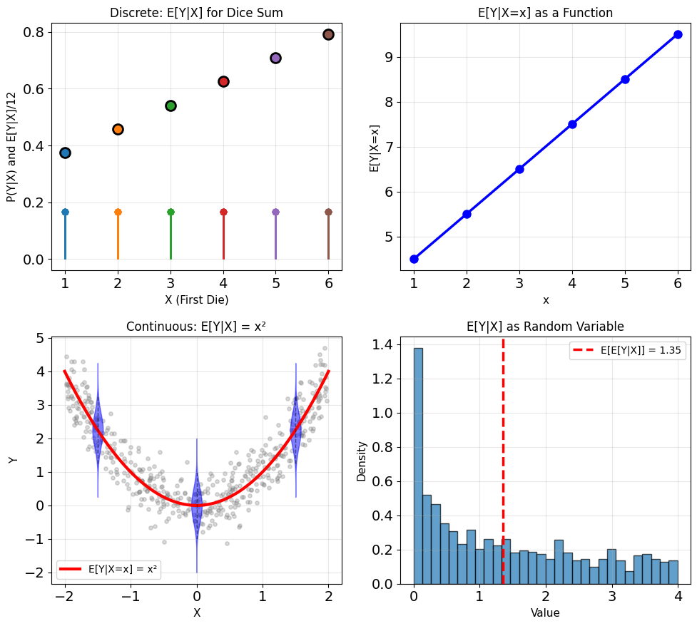
- \(\mathbb{E}[Y|X=x]\) is a number (for fixed \(x\))
- expected value when \(X\) equals \(x\)
- \(g(x) = \mathbb{E}[Y|X=x]\) is a deterministic function
- \(\mathbb{E}[Y|X]\) is a random variable (function of \(X\))
Example: \(Y = X + N\), \(N \sim \mathcal{N}(0,1)\), independent \(X\) and \(N\)
\[\mathbb{E}[Y|X=x] = \mathbb{E}[x + N] = x\]
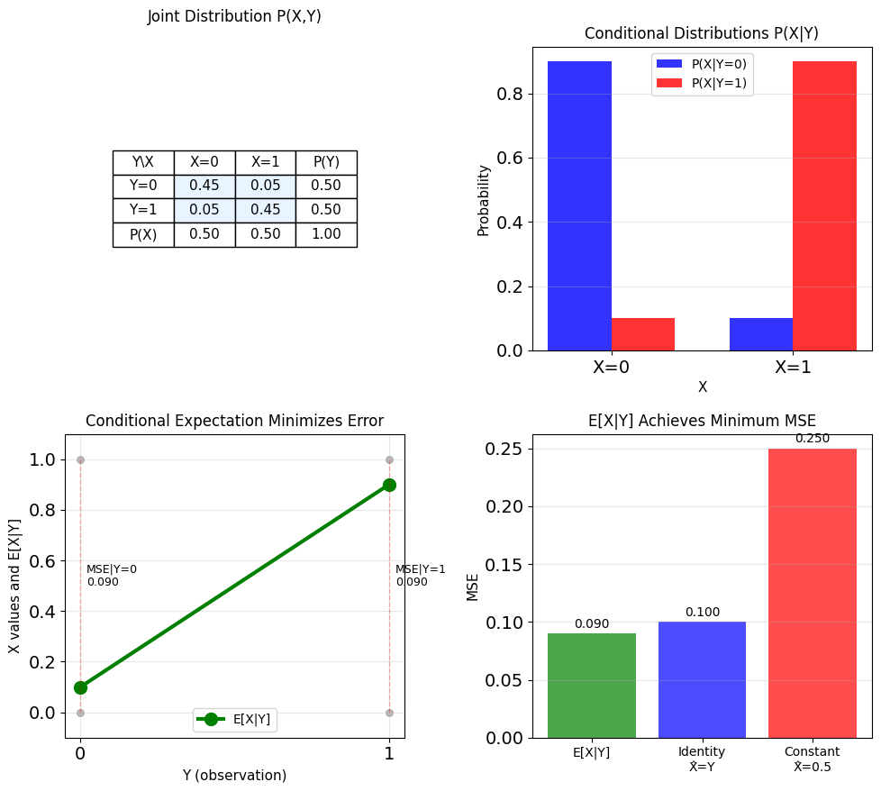
Binary Channel: \(\mathbb{E}[X|Y]\) Achieves Minimum MSE
Example: Binary communication channel
- \(X \in \{0, 1\}\): transmitted bit
- \(Y \in \{0, 1\}\): received bit
- Channel flips bit with probability \(p = 0.1\)
Joint distribution:
\[P(X=0, Y=0) = 0.45, \quad P(X=1, Y=0) = 0.05\]
\[P(X=0, Y=1) = 0.05, \quad P(X=1, Y=1) = 0.45\]
Conditional distributions:
\[P(X=0|Y=0) = \frac{0.45}{0.5} = 0.9\]
\[P(X=1|Y=0) = \frac{0.05}{0.5} = 0.1\]
Conditional expectations:
\[\mathbb{E}[X|Y=0] = 0 \cdot 0.9 + 1 \cdot 0.1 = 0.1\]
\[\mathbb{E}[X|Y=1] = 0 \cdot 0.1 + 1 \cdot 0.9 = 0.9\]
MSE for different predictors:
- \(\hat{X} = \mathbb{E}[X|Y]\): MSE = 0.09
- \(\hat{X} = Y\) (identity): MSE = 0.10
- \(\hat{X} = 0.5\) (constant): MSE = 0.25
Result: \(\mathbb{E}[X|Y]\) achieves minimum MSE
Gaussian Conditional Mean Is Linear in \(X\)
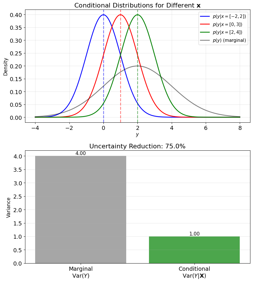
Joint Gaussian: \((X, Y) \sim \mathcal{N}(\mu, K)\)
Parameters:
\[\mu = \begin{bmatrix} \mu_X \\ \mu_Y \end{bmatrix}, \quad K = \begin{bmatrix} \sigma_X^2 & \rho\sigma_X\sigma_Y \\ \rho\sigma_X\sigma_Y & \sigma_Y^2 \end{bmatrix}\]
Conditional mean:
\[\mathbb{E}[Y|X=x] = \mu_Y + \rho\frac{\sigma_Y}{\sigma_X}(x - \mu_X)\]
Conditional variance:
\[\text{Var}(Y|X=x) = \sigma_Y^2(1 - \rho^2)\]
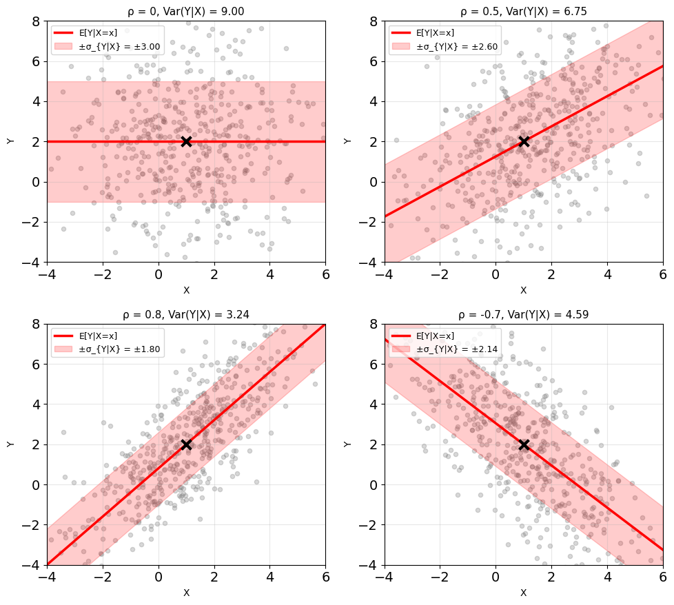
Linear in \(x\), spread independent of \(x\)
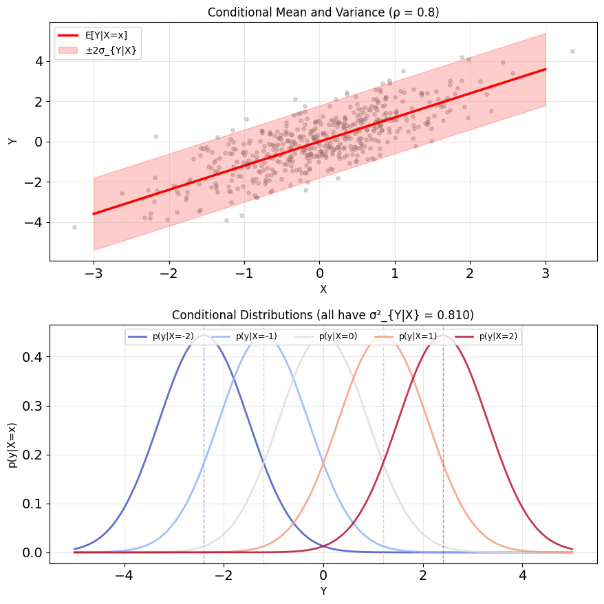
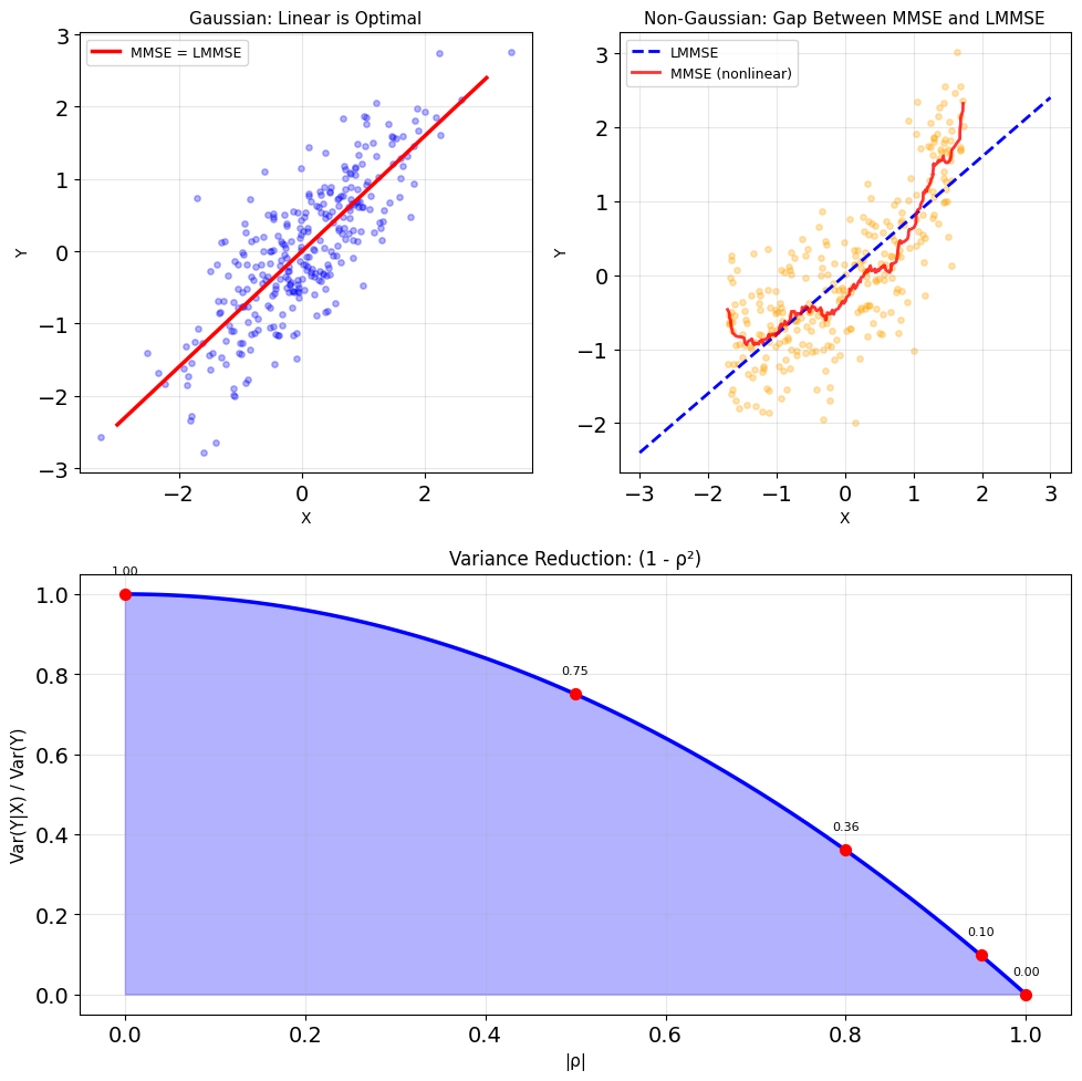
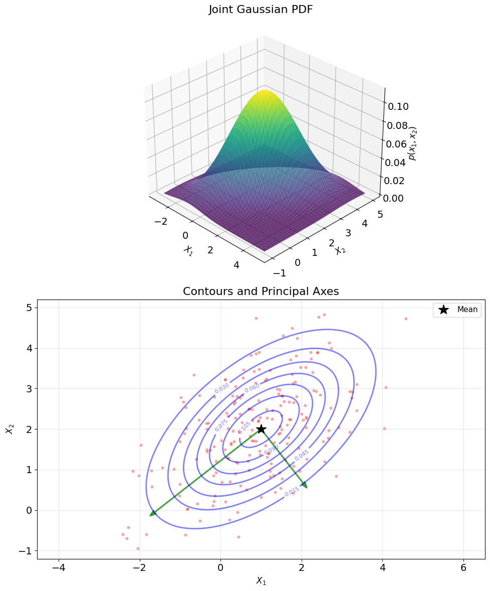
Figure: \(\mu = (1, 2)\), \(\sigma_X = 2\), \(\sigma_Y = 3\); at \(\rho = 0.8\) the slope is \(1.2\) and the spread \(1.8\), at \(\rho = 0\) the slope is \(0\) and the spread the full \(3\)
Need the Conditional Density to Compute \(\mathbb{E}[Y|X]\)
Computing \(\mathbb{E}[Y|X=x]\) requires \(p(y|x)\)
From Bayes:
\[p(y|x) = \frac{p(x,y)}{p(x)} = \frac{p(x|y)p(y)}{\int p(x|y')p(y')dy'}\]
When tractable:
- Known parametric families (Gaussian, exponential)
- Discrete with small state space
- Special structures (independence, Markov)
When intractable (often no closed form):
- Complex nonlinear relationships
- High dimensions
- Unknown distributions
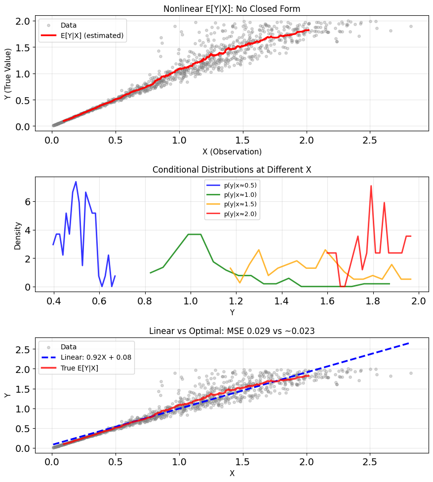
Example: Nonlinear sensor
\[Y = \text{true value}, \quad X = Y + Y^2 \cdot N\]
where \(N \sim \mathcal{N}(0, 0.1)\)
Computing \(\mathbb{E}[Y|X=x]\) requires:
- Joint density \(p(x,y)\)
- Marginal \(p(x) = \int p(x,y)dy\)
- Conditional \(p(y|x) = p(x,y)/p(x)\)
- Integration \(\mathbb{E}[Y|X=x] = \int y p(y|x) dy\)
Iterated Expectations Recover the Mean
Law of Total Expectation:
\[\mathbb{E}[\mathbb{E}[Y|X]] = \mathbb{E}[Y]\]
Proof:
\[\mathbb{E}[\mathbb{E}[Y|X]] = \mathbb{E}[g(X)]\]
where \(g(x) = \mathbb{E}[Y|X=x]\)
\[= \int g(x) p(x) dx = \int \mathbb{E}[Y|X=x] p(x) dx\]
\[= \int \left(\int y \, p(y|x) dy\right) p(x) dx\]
\[= \int\int y \, p(y|x) p(x) dy \, dx\]
\[= \int y \left(\int p(y|x)p(x) dx\right) dy\]
\[= \int y \, p(y) dy = \mathbb{E}[Y]\]
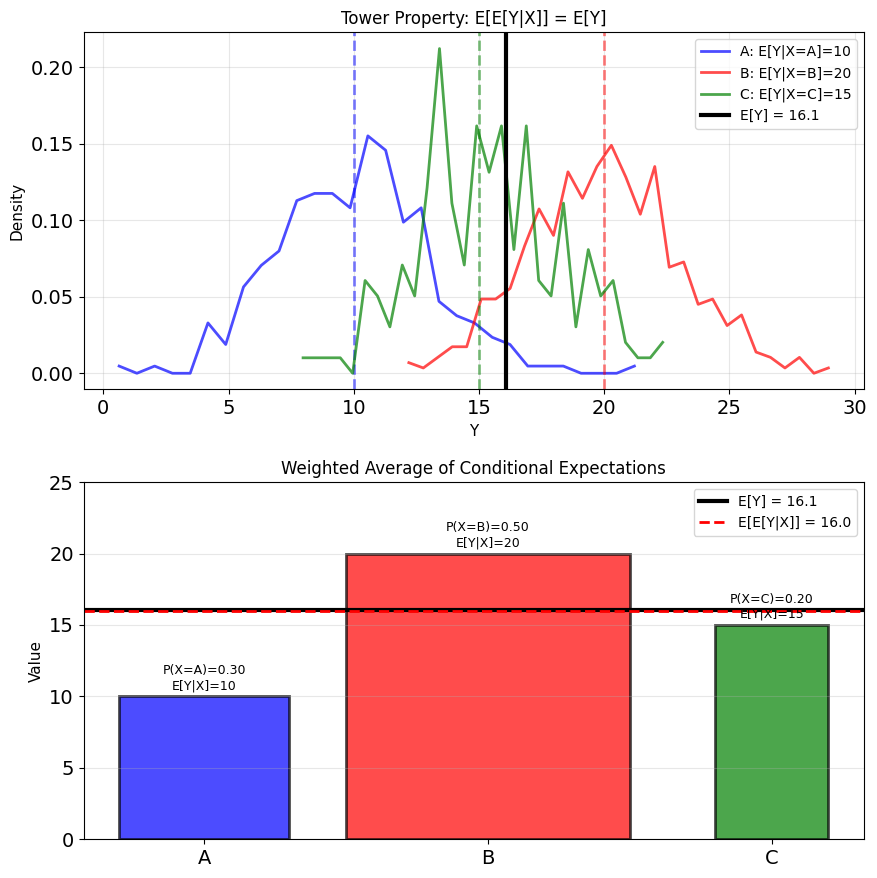
Intuition: Average of conditional averages = unconditional average
Example: Class grades
- Section A: mean 85, 30 students
- Section B: mean 75, 20 students
- Overall mean = \(\frac{30 \cdot 85 + 20 \cdot 75}{50} = 81\)
Functions of \(X\) Factor Out
Property: For any function \(h(X)\):
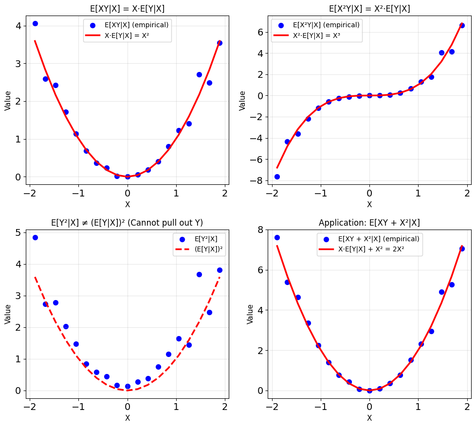
\[\mathbb{E}[h(X)Y | X] = h(X)\mathbb{E}[Y|X]\]
Proof: Fix \(X = x\). Then \(h(X) = h(x)\) is a constant:
\[\mathbb{E}[h(X)Y | X=x] = \mathbb{E}[h(x)Y | X=x]\]
\[= h(x)\mathbb{E}[Y | X=x]\]
Special cases:
- \(\mathbb{E}[X \cdot Y | X] = X \cdot \mathbb{E}[Y|X]\)
- \(\mathbb{E}[f(X) + Y | X] = f(X) + \mathbb{E}[Y|X]\)
- \(\mathbb{E}[X^2Y | X] = X^2\mathbb{E}[Y|X]\)
Example: Signal processing
\[Z = X \cdot Y + X^2\]
\[\mathbb{E}[Z|X] = X\mathbb{E}[Y|X] + X^2\]
Only \(\mathbb{E}[Y|X]\) is needed, not \(\mathbb{E}[XY|X]\)
But functions of \(Y\) do not factor out:
\[\mathbb{E}[Y^2|X] \neq (\mathbb{E}[Y|X])^2\]
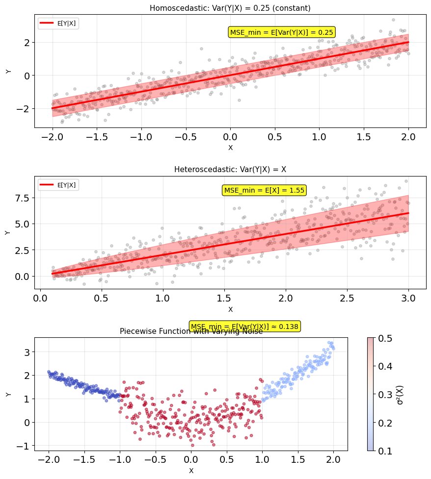
Var(Y|X) Is Irreducible Uncertainty
Definition:
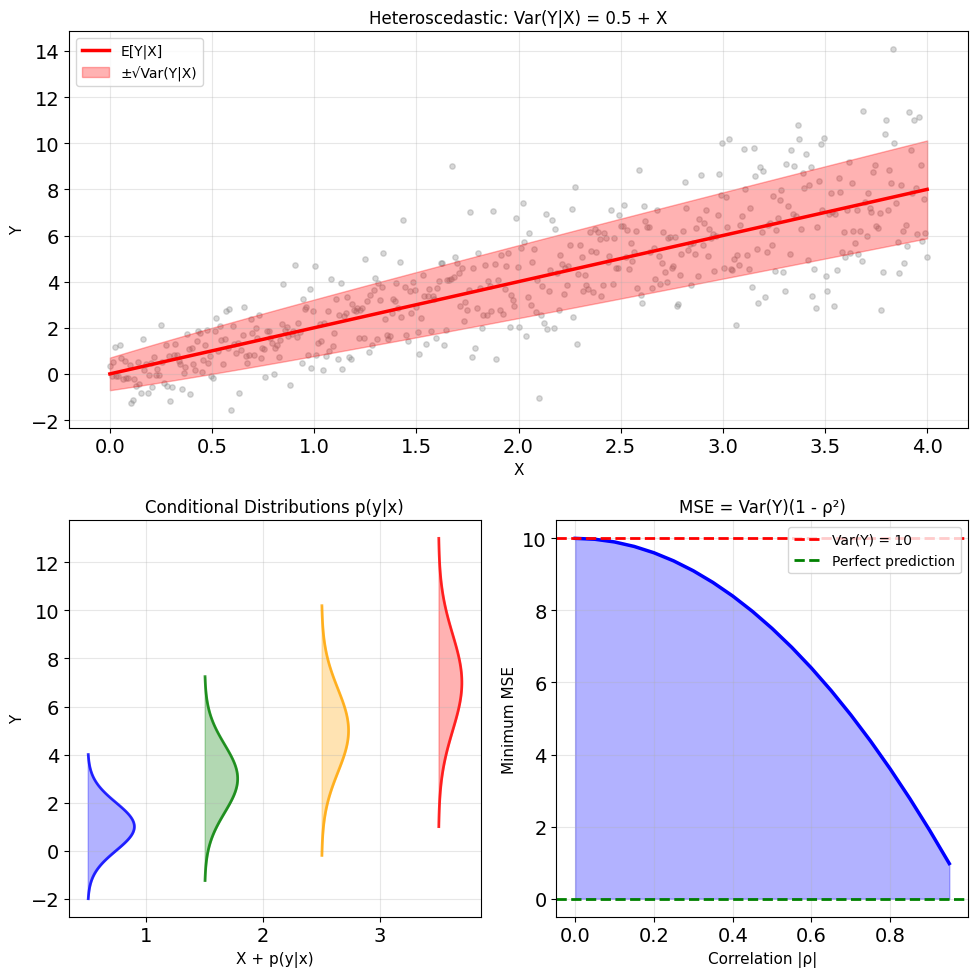
\[\text{Var}(Y|X) = \mathbb{E}[(Y - \mathbb{E}[Y|X])^2 | X]\]
Computing formula:
\[\text{Var}(Y|X) = \mathbb{E}[Y^2|X] - (\mathbb{E}[Y|X])^2\]
Measures remaining uncertainty after observing \(X\)
Law of Total Variance:
\[\text{Var}(Y) = \mathbb{E}[\text{Var}(Y|X)] + \text{Var}(\mathbb{E}[Y|X])\]
- First term: Average conditional variance (irreducible)
- Second term: Variance of conditional means (explained)
Interpretation:
\[\text{Total uncertainty} = \text{Unexplained} + \text{Explained by } X\]
Minimum MSE: \(\mathbb{E}[\text{Var}(Y|X)]\), and no predictor does better
MMSE Optimization Is Infinite-Dimensional
Goal: Find the best predictor of \(Y\) given \(X\)
Function space:
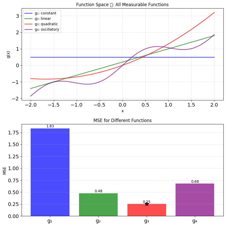
\[\mathcal{G} = \{g: \mathbb{R} \to \mathbb{R} \text{ measurable}\}\]
Optimization problem:
\[\min_{g \in \mathcal{G}} \text{MSE}(g) = \min_{g \in \mathcal{G}} \mathbb{E}[(Y - g(X))^2]\]
Infinite-dimensional optimization
- Search over all possible functions
- No parametric form assumed
- No finite parameter vector to solve for
Strategy: Decompose the problem by conditioning on \(X\)
- Fix \(X = x\), solve pointwise optimization
- Combine solutions for all \(x\)
- Verify global optimality
Conditioning Decomposes MSE into Subproblems
Decomposition:
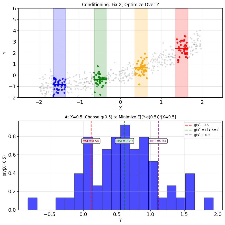
\[\text{MSE}(g) = \mathbb{E}[(Y - g(X))^2] = \mathbb{E}[\mathbb{E}[(Y - g(X))^2|X]]\]
Why this helps:
- Outside expectation: Average over \(X\)
- Inside expectation: For each fixed \(X = x\)
When \(X = x\) is fixed:
- \(g(X) = g(x)\) is just a number
- \(Y|X=x\) has distribution \(p(y|x)\)
- We minimize: \(\mathbb{E}[(Y - g(x))^2|X=x]\)
This transforms the problem:
- From: Find optimal function \(g\)
- To: For each \(x\), find optimal constant \(g(x)\)
Solution approach:
- Fix \(x\), find best constant predictor
- This gives us \(g^*(x)\) for each \(x\)
- The function \(g^*\) is our MMSE estimator
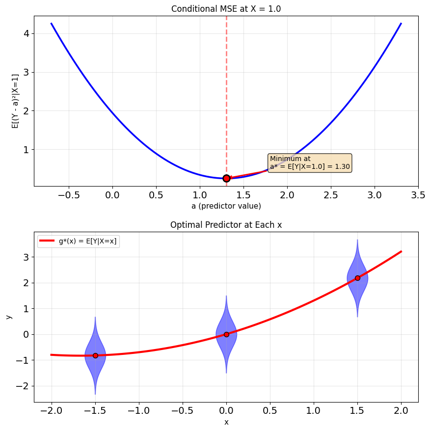
First-Order Condition Yields \(\mathbb{E}[Y|X]\)
Step 1: Express MSE using conditional expectation
\[\text{MSE}(g) = \mathbb{E}[(Y - g(X))^2]\]
\[= \mathbb{E}[\mathbb{E}[(Y - g(X))^2|X]]\]
Step 2: For fixed \(X = x\), \(g(X) = g(x)\) is a constant
\[\mathbb{E}[(Y - g(x))^2|X=x] = \mathbb{E}[(Y - a)^2|X=x]\]
where \(a = g(x)\)
Step 3: Minimize over \(a\)
\[\frac{d}{da}\mathbb{E}[(Y - a)^2|X=x] = 0\]
\[-2\mathbb{E}[(Y - a)|X=x] = 0\]
\[\mathbb{E}[Y|X=x] - a = 0\]
Solution: \(a^* = \mathbb{E}[Y|X=x]\)
Step 4: Since this holds for all \(x\):
\[g^*(x) = \mathbb{E}[Y|X=x]\]
Therefore:
\[\boxed{\hat{Y}_{\text{MMSE}} = \mathbb{E}[Y|X]}\]
Optimal Error Is Uncorrelated with \(h(X)\)
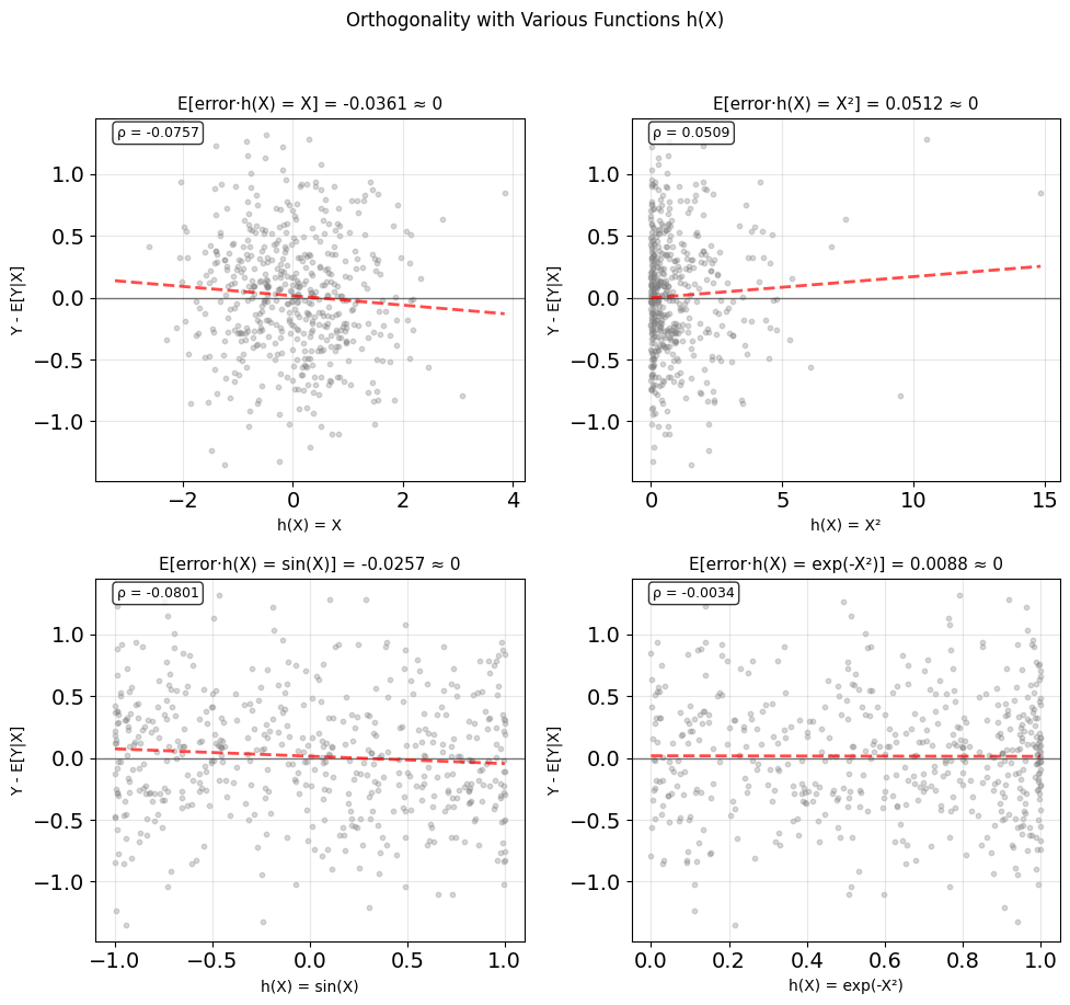
Orthogonality principle: Optimal error orthogonal to any function of \(X\):
\[\mathbb{E}[(Y - \mathbb{E}[Y|X])h(X)] = 0\]
for any measurable \(h\).
-
Uniqueness: Only one function satisfies this \(\Rightarrow\) unique MMSE
-
Optimality test: If \(\mathbb{E}[\epsilon \cdot h(X)] \neq 0\), can reduce MSE by adjusting estimate in direction of \(h(X)\)
-
Computational foundation:
- Linear case \(\to\) normal equations
- Adaptive filters \(\to\) orthogonalize error
- Kalman filter \(\to\) innovation orthogonality
-
Geometric meaning: MMSE = projection in Hilbert space
Proof: \(\mathbb{E}[(Y - \mathbb{E}[Y|X])|X] = 0\) by definition, multiplying by \(h(X)\) preserves this.
Cannot extract more information from \(X\)
Pointwise Optimality Implies Global Optimality
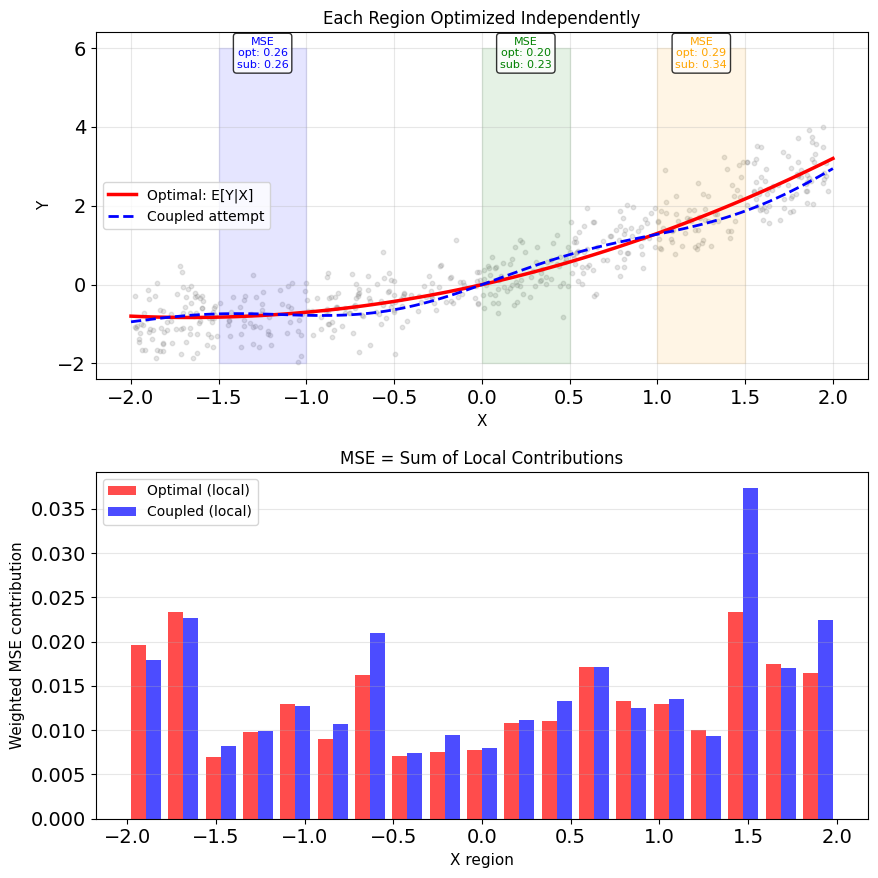
We solved pointwise: For each \(x\), found \(g^*(x) = \mathbb{E}[Y|X=x]\)
Question: Is this globally optimal over all functions?
Two concerns:
- We optimized separately at each \(x\)
- Maybe coupling across different \(x\) values helps?
MSE decomposes additively
\[\text{MSE}(g) = \int \mathbb{E}[(Y - g(x))^2|X=x] p(x) dx\]
Each term \(\mathbb{E}[(Y - g(x))^2|X=x]\) depends only on \(g(x)\), not on \(g(x')\) for \(x' \neq x\).
Therefore:
- Minimizing each term separately minimizes the sum
- No coupling can improve the solution
- Pointwise optimization = Global optimization
Idea: Prediction at \(x\) doesn’t help prediction at \(x'\)
Suboptimal Predictors Add Excess MSE
Claim: No function can beat \(\mathbb{E}[Y|X]\)
Proof: For any function \(g\):
\[\text{MSE}(g) = \mathbb{E}[(Y - g(X))^2]\]
Add and subtract \(\mathbb{E}[Y|X]\):
\[= \mathbb{E}[(Y - \mathbb{E}[Y|X] + \mathbb{E}[Y|X] - g(X))^2]\]
Expand the square:
\[= \mathbb{E}[(Y - \mathbb{E}[Y|X])^2] + \mathbb{E}[(\mathbb{E}[Y|X] - g(X))^2]\]
\[+ 2\mathbb{E}[(Y - \mathbb{E}[Y|X])(\mathbb{E}[Y|X] - g(X))]\]
The cross term vanishes:
\[\mathbb{E}[(Y - \mathbb{E}[Y|X])(\mathbb{E}[Y|X] - g(X))] = 0\]
Because \(\mathbb{E}[Y|X] - g(X)\) is a function of \(X\) and:
\[\mathbb{E}[(Y - \mathbb{E}[Y|X])h(X)] = 0\]
for any \(h(X)\) (orthogonality).
Therefore:
\[\text{MSE}(g) = \text{MSE}_{\min} + \mathbb{E}[(\mathbb{E}[Y|X] - g(X))^2] \geq \text{MSE}_{\min}\]
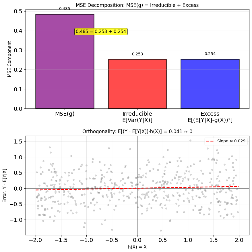
MSE\(_{\min}\) = \(\mathbb{E}[\text{Var}(Y|X)]\)
Minimum achievable MSE:
\[\text{MSE}_{\min} = \mathbb{E}[(Y - \mathbb{E}[Y|X])^2]\]
Result:
\[\boxed{\text{MSE}_{\min} = \mathbb{E}[\text{Var}(Y|X)]}\]
Proof:
\[\text{MSE}_{\min} = \mathbb{E}[(Y - \mathbb{E}[Y|X])^2]\]
\[= \mathbb{E}[\mathbb{E}[(Y - \mathbb{E}[Y|X])^2|X]]\]
For fixed \(X = x\):
\[\mathbb{E}[(Y - \mathbb{E}[Y|X=x])^2|X=x] = \text{Var}(Y|X=x)\]
Therefore:
\[\text{MSE}_{\min} = \mathbb{E}[\text{Var}(Y|X)]\]
Irreducible: no predictor can remove conditional variance
Special cases:
- \(X\) and \(Y\) independent: \(\text{MSE}_{\min} = \text{Var}(Y)\)
- \(Y = f(X)\) deterministic: \(\text{MSE}_{\min} = 0\)
Squared Error Makes MMSE Outlier-Sensitive
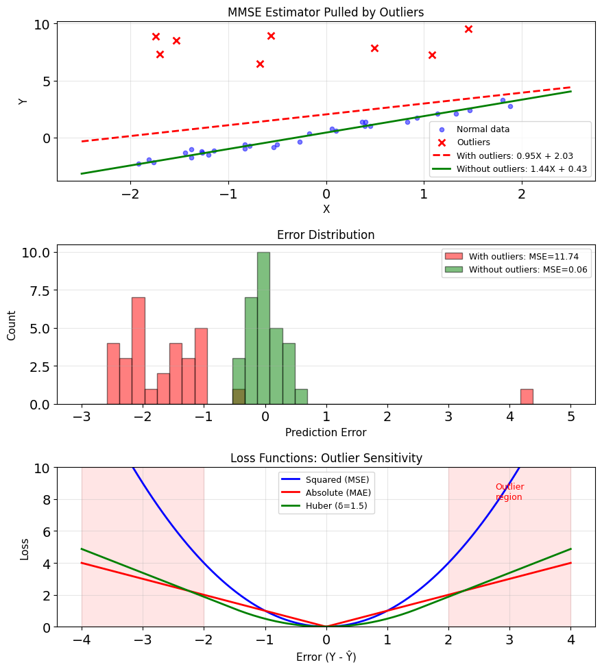
A single outlier can dominate the sample MSE:
\[\widehat{\text{MSE}} = \frac{1}{n}\sum_{i=1}^n (y_i - \hat{y}_i)^2\]
If \(y_k\) is an outlier: \((y_k - \hat{y}_k)^2 \gg (y_i - \hat{y}_i)^2\) for \(i \neq k\)
Effect on the estimate:
- Under contamination, the conditional mean shifts toward the outlier component
- The fit stops representing the majority of data
Example: Sensor failure
- 99 readings: \(Y \approx X + \varepsilon\), \(\varepsilon \sim \mathcal{N}(0, 0.1^2)\)
- 1 reading: \(Y = 100\) (sensor spike)
The mean absorbs the spike; typical-case error grows.
Alternative loss functions:
- Absolute error: \(|Y - \hat{Y}|\) (median)
- Huber loss: Quadratic for small errors, linear for large
- Trimmed MSE: Ignore largest errors
Median Regression Is Robust to Outliers
When outliers are present:
-
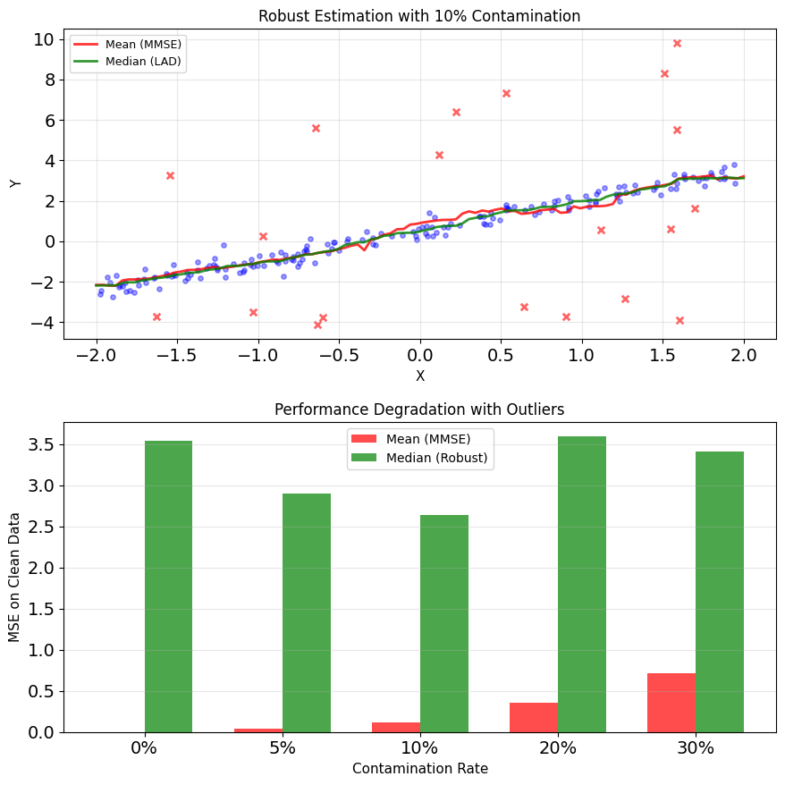
Median regression (LAD):
\[\min_g \mathbb{E}[|Y - g(X)|]\]Solution: \(g^*(x) = \text{median}(Y|X=x)\)
-
Huber regression:
\[\min_g \mathbb{E}[\ell_\delta(Y - g(X))]\]where \(\ell_\delta(e) = \begin{cases} \frac{1}{2}e^2 & |e| \leq \delta \\ \delta|e| - \frac{\delta^2}{2} & |e| > \delta \end{cases}\)
-
Trimmed mean: Remove top/bottom α% before computing \(\mathbb{E}[Y|X]\)
Inner Products Measure Alignment
Definition: For vectors \(\mathbf{x}, \mathbf{y} \in \mathbb{R}^n\)
\[\langle \mathbf{x}, \mathbf{y} \rangle = \mathbf{x}^T\mathbf{y} = \sum_{i=1}^n x_i y_i\]
Geometric interpretation:
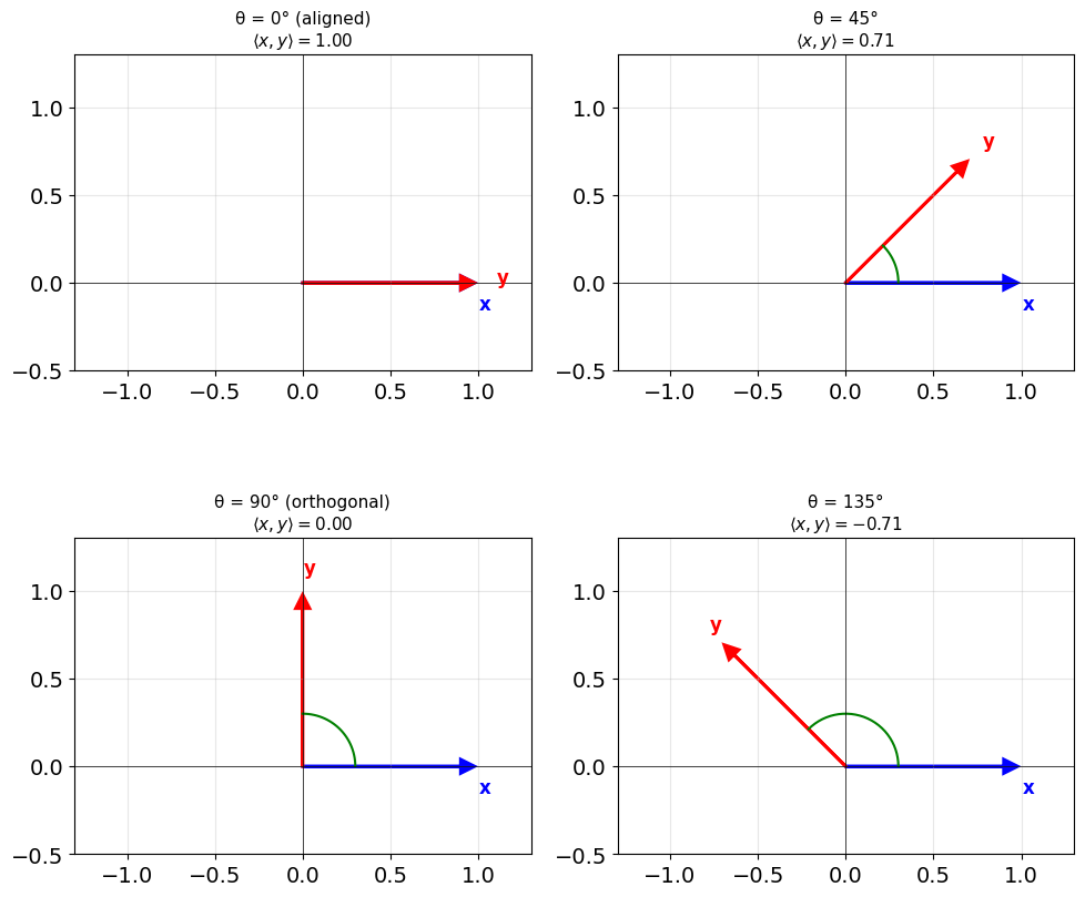
\[\langle \mathbf{x}, \mathbf{y} \rangle = \|\mathbf{x}\| \|\mathbf{y}\| \cos\theta\]
where \(\theta\) is the angle between vectors.
Special cases:
- \(\theta = 0^\circ\): \(\langle \mathbf{x}, \mathbf{y} \rangle = \|\mathbf{x}\|\|\mathbf{y}\|\) (aligned)
- \(\theta = 90^\circ\): \(\langle \mathbf{x}, \mathbf{y} \rangle = 0\) (orthogonal)
- \(\theta = 180^\circ\): \(\langle \mathbf{x}, \mathbf{y} \rangle = -\|\mathbf{x}\|\|\mathbf{y}\|\) (opposed)
Norm from inner product:
\[\|\mathbf{x}\| = \sqrt{\langle \mathbf{x}, \mathbf{x} \rangle} = \sqrt{\sum_i x_i^2}\]
Projection Finds the Closest Point in a Subspace
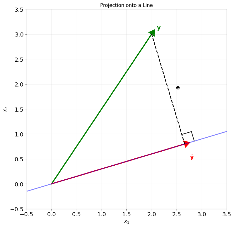
Problem: Given \(\mathbf{y}\) and subspace \(\mathcal{S}\), find \(\hat{\mathbf{y}} \in \mathcal{S}\) that minimizes
\[\|\mathbf{y} - \hat{\mathbf{y}}\|^2\]
Solution: \(\hat{\mathbf{y}} = \text{Proj}_{\mathcal{S}}(\mathbf{y})\)
Projection onto a line (1D subspace):
Given direction \(\mathbf{u}\) with \(\|\mathbf{u}\| = 1\):
\[\hat{\mathbf{y}} = \langle \mathbf{y}, \mathbf{u} \rangle \mathbf{u}\]
Projection onto span of \(\{\mathbf{u}_1, \mathbf{u}_2\}\):
If \(\mathbf{u}_1 \perp \mathbf{u}_2\) and both unit vectors:
\[\hat{\mathbf{y}} = \langle \mathbf{y}, \mathbf{u}_1 \rangle \mathbf{u}_1 + \langle \mathbf{y}, \mathbf{u}_2 \rangle \mathbf{u}_2\]
The error is what remains:
\[\mathbf{e} = \mathbf{y} - \hat{\mathbf{y}}\]
Orthogonal Error = Minimum Distance
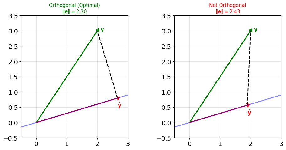
Theorem: \(\hat{\mathbf{y}}\) minimizes \(\|\mathbf{y} - \hat{\mathbf{y}}\|^2\) over \(\mathcal{S}\)
if and only if
\[(\mathbf{y} - \hat{\mathbf{y}}) \perp \mathcal{S}\]
Why orthogonality implies optimality:
Suppose error \(\mathbf{e} = \mathbf{y} - \hat{\mathbf{y}}\) is not orthogonal to \(\mathcal{S}\).
Then \(\mathbf{e}\) has a component along \(\mathcal{S}\).
Moving \(\hat{\mathbf{y}}\) in that direction reduces \(\|\mathbf{e}\|\).
Contradiction: \(\hat{\mathbf{y}}\) wasn’t optimal.
Orthogonality conditions:
For \(\mathcal{S} = \text{span}\{\mathbf{v}_1, ..., \mathbf{v}_k\}\):
\[\langle \mathbf{y} - \hat{\mathbf{y}}, \mathbf{v}_i \rangle = 0 \quad \text{for } i = 1, ..., k\]
This gives \(k\) equations to solve for \(\hat{\mathbf{y}}\).
\(\mathbb{E}[XY]\) Is an Inner Product
Random variable inner product:
Define \(\langle X, Y \rangle = \mathbb{E}[XY]\)
For zero-mean variables:
\[\langle X, Y \rangle = \mathbb{E}[XY] = \text{Cov}(X, Y)\]
Orthogonal random variables:
\[X \perp Y \iff \mathbb{E}[XY] = 0\]
(For zero-mean: \(\text{Cov}(X,Y) = 0\))
The connection:
| Vectors | Random Variables |
|---|---|
| \(\langle \mathbf{x}, \mathbf{y} \rangle = \mathbf{x}^T\mathbf{y}\) | \(\langle X, Y \rangle = \mathbb{E}[XY]\) |
| \(\mathbf{x} \perp \mathbf{y}\) | \(X \perp Y\) |
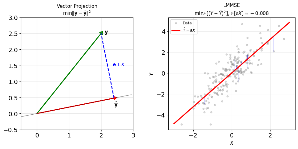
| Projection minimizes \(|\mathbf{y} - \hat{\mathbf{y}}|^2\) | LMMSE minimizes \(\mathbb{E}[(Y - \hat{Y})^2]\) |
| Error \(\perp\) subspace | Error \(\perp\) predictors |
This is why linear algebra solves estimation problems.
Density Estimation Needs Exponential Samples
Curse of dimensionality:
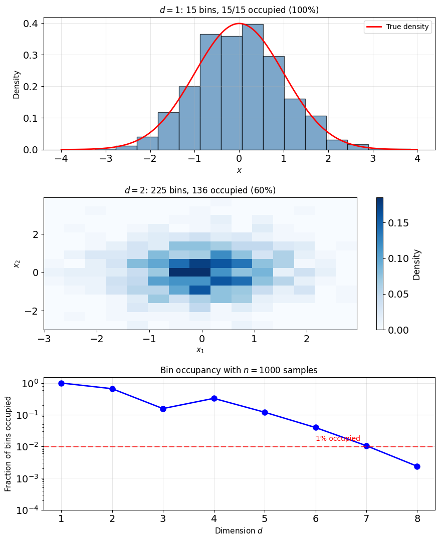
To compute \(\mathbb{E}[Y|X]\), need \(p(y|x)\)
Density estimation convergence:
- Rate: \(N^{-4/(d+4)}\) for \(d\)-dimensional data
- 10% relative error: \(d{=}10 \to N \approx 10^6\); \(d{=}100 \to N \approx 10^{26}\)
Consequence:
- Modern data is high-dimensional
- Never have enough samples for nonparametric methods
- Must accept suboptimality for tractability
Linear class advantages:
- Only need second moments: \(O(d^2)\) parameters
- Sample complexity: \(O(d^2)\) vs \(O(e^d)\)
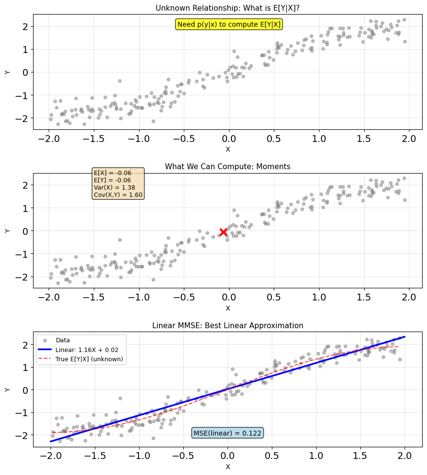
Data Gives Moments, Not Densities
MMSE requires \(p(y|x)\) to compute \(\mathbb{E}[Y|X]\)
Reality: We rarely know conditional distributions
What we often have:
- Sample data: \((x_1, y_1), ..., (x_n, y_n)\)
- First and second moments
Practical solution: Restrict to linear predictors
\[\hat{Y} = aX + b\]
- Only need means, variances, covariance
- Optimal for Gaussian
- Optimal whenever \(\mathbb{E}[Y|X]\) is linear
Two Parameters Instead of \(\infty\)
Function class:
\[\mathcal{L} = \{g(x) = ax + b : a, b \in \mathbb{R}\}\]
New optimization problem:
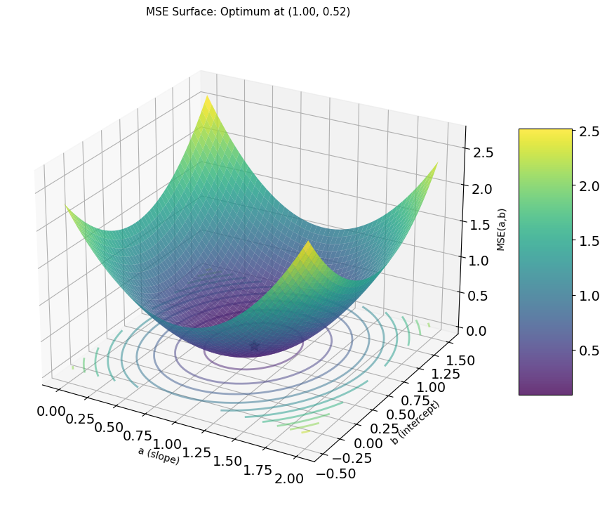
\[\min_{a,b} \text{MSE}(a,b) = \min_{a,b} \mathbb{E}[(Y - aX - b)^2]\]
From infinite to finite:
- Before: Search over all functions
- Now: Search over 2 parameters
Expanding the MSE:
\[\text{MSE}(a,b) = \mathbb{E}[Y^2 - 2Y(aX + b) + (aX + b)^2]\]
\[= \mathbb{E}[Y^2] - 2a\mathbb{E}[XY] - 2b\mathbb{E}[Y]\]
\[+ a^2\mathbb{E}[X^2] + 2ab\mathbb{E}[X] + b^2\]
MSE is quadratic in \((a, b)\)
- Unique minimum (if Var\((X) > 0\))
- Closed-form solution via derivatives
- No iterative optimization needed
Optimal Offset Forces Zero Mean Error
Step 1: Find optimal \(b\) for fixed \(a\)
Take derivative with respect to \(b\):
\[\frac{\partial}{\partial b}\text{MSE}(a,b) = \frac{\partial}{\partial b}\mathbb{E}[(Y - aX - b)^2]\]
\[= -2\mathbb{E}[Y - aX - b] = 0\]
Solving for \(b\):
\[\mathbb{E}[Y - aX - b] = 0\]
\[\mathbb{E}[Y] - a\mathbb{E}[X] - b = 0\]
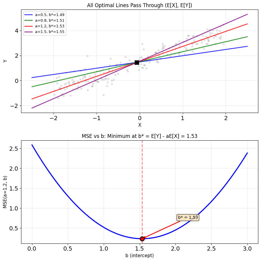
\[\boxed{b^* = \mathbb{E}[Y] - a\mathbb{E}[X]}\]
Interpretation:
- Offset ensures zero mean error
- Forces predictor through \((\mathbb{E}[X], \mathbb{E}[Y])\)
- Adjusts for non-zero means
Substituting back:
\[\hat{Y} = aX + \mathbb{E}[Y] - a\mathbb{E}[X] = \mathbb{E}[Y] + a(X - \mathbb{E}[X])\]
Optimal Slope = \(\text{Cov}(X,Y)/\text{Var}(X)\)
Step 2: Find optimal \(a\) using \(b^* = \mathbb{E}[Y] - a\mathbb{E}[X]\)
Substitute into MSE:
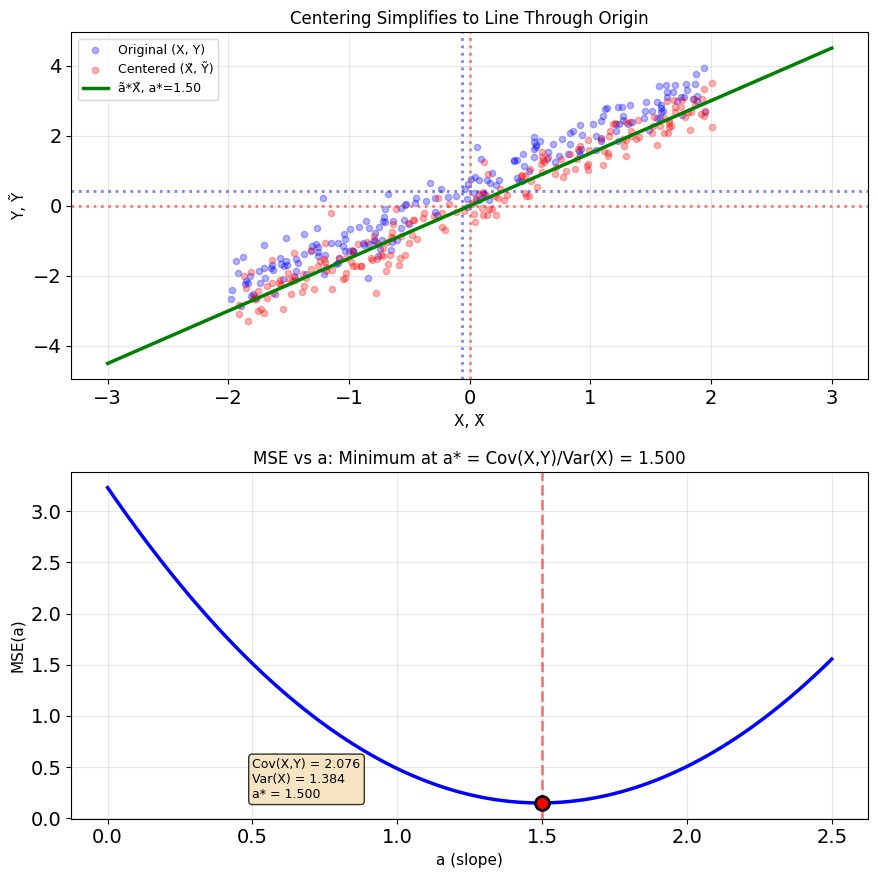
\[\text{MSE}(a) = \mathbb{E}[(Y - \mathbb{E}[Y] - a(X - \mathbb{E}[X]))^2]\]
Define centered variables:
- \(\tilde{Y} = Y - \mathbb{E}[Y]\)
- \(\tilde{X} = X - \mathbb{E}[X]\)
Then: \(\text{MSE}(a) = \mathbb{E}[(\tilde{Y} - a\tilde{X})^2]\)
Take derivative:
\[\frac{d}{da}\text{MSE}(a) = -2\mathbb{E}[\tilde{X}(\tilde{Y} - a\tilde{X})] = 0\]
\[\mathbb{E}[\tilde{X}\tilde{Y}] - a\mathbb{E}[\tilde{X}^2] = 0\]
Solution:
\[\boxed{a^* = \frac{\mathbb{E}[\tilde{X}\tilde{Y}]}{\mathbb{E}[\tilde{X}^2]} = \frac{\text{Cov}(X,Y)}{\text{Var}(X)}}\]
Note: \(\mathbb{E}[\tilde{X}\tilde{Y}] = \text{Cov}(X,Y)\) and \(\mathbb{E}[\tilde{X}^2] = \text{Var}(X)\)
Orthogonality Recovers the Slope Without Calculus
Alternative approach: Require error orthogonal to predictors
From MMSE theory: optimal error satisfies
\[\mathbb{E}[(Y - \hat{Y}) \cdot h(X)] = 0\]
for functions \(h\) in the predictor class.
For linear predictors \(\hat{Y} = aX + b\):
Predictor class = span\(\{1, X\}\)
Orthogonality conditions:
-
\(\mathbb{E}[(Y - aX - b) \cdot 1] = 0\)
\[\mathbb{E}[Y] - a\mathbb{E}[X] - b = 0\]\[\boxed{b = \mathbb{E}[Y] - a\mathbb{E}[X]}\] -
\(\mathbb{E}[(Y - aX - b) \cdot X] = 0\)
\[\mathbb{E}[XY] - a\mathbb{E}[X^2] - b\mathbb{E}[X] = 0\]
Substitute \(b\) and solve:
\[\boxed{a = \frac{\text{Cov}(X,Y)}{\text{Var}(X)}}\]
Same answer, different route
- Calculus: minimize MSE directly
- Orthogonality: project onto subspace
Orthogonality generalizes to vectors without derivatives.
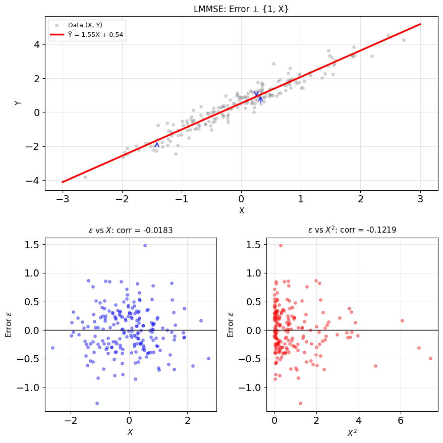
LMMSE Needs Only Means and Covariances
Complete solution:
\[\boxed{\hat{Y}_{\text{LMMSE}} = \mathbb{E}[Y] + \frac{\text{Cov}(X,Y)}{\text{Var}(X)}(X - \mathbb{E}[X])}\]
Alternative forms:
Using correlation \(\rho = \frac{\text{Cov}(X,Y)}{\sigma_X \sigma_Y}\):
\[\hat{Y}_{\text{LMMSE}} = \mathbb{E}[Y] + \rho\frac{\sigma_Y}{\sigma_X}(X - \mathbb{E}[X])\]
Standardized form: If \(\mathbb{E}[X] = \mathbb{E}[Y] = 0\) and \(\sigma_X = \sigma_Y = 1\):
\[\hat{Y}_{\text{LMMSE}} = \rho X\]
Minimum MSE:
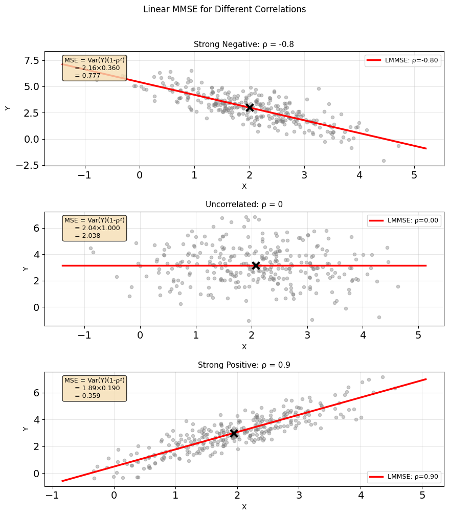
\[\text{MSE}_{\text{LMMSE}} = \text{Var}(Y)(1 - \rho^2)\]
Explained variance:
\[\rho^2 = \frac{\text{Var}(Y) - \text{MSE}_{\text{LMMSE}}}{\text{Var}(Y)}\]
Correlation measures linear predictability, not dependence
Properties:
- Only needs first and second moments
- Always exists (if Var\((X) > 0\))
- Unique solution
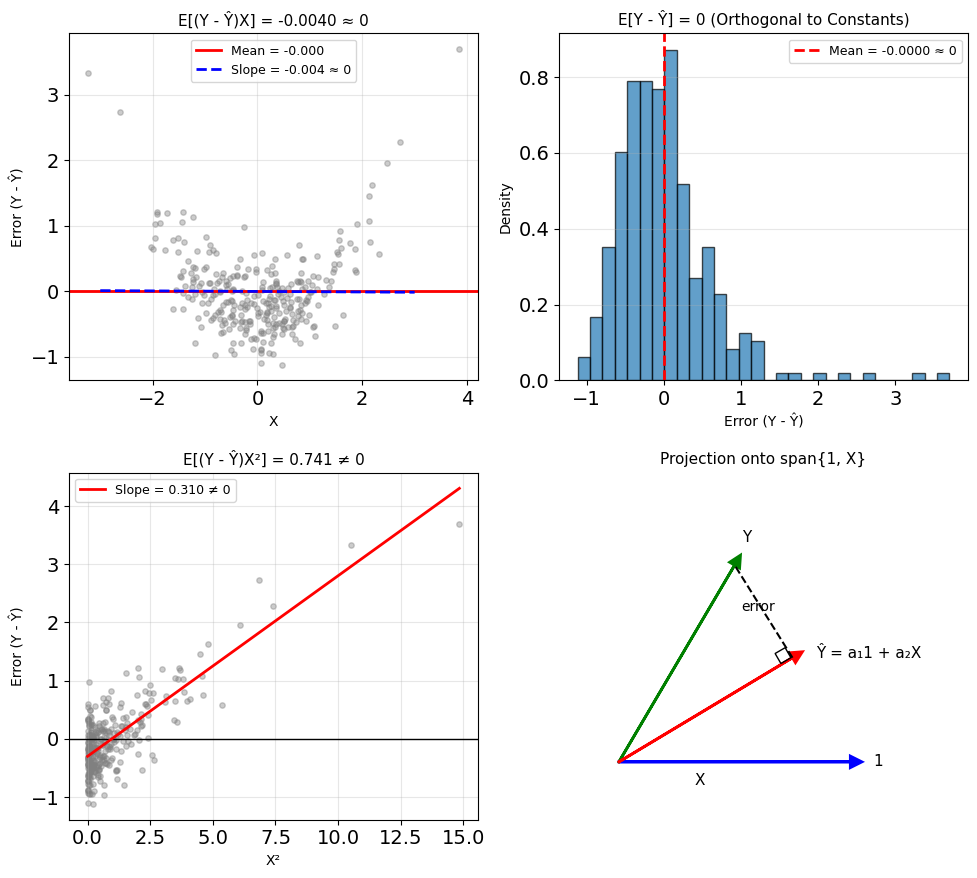
- Orthogonal errors: \(\mathbb{E}[(Y - \hat{Y})X] = 0\)
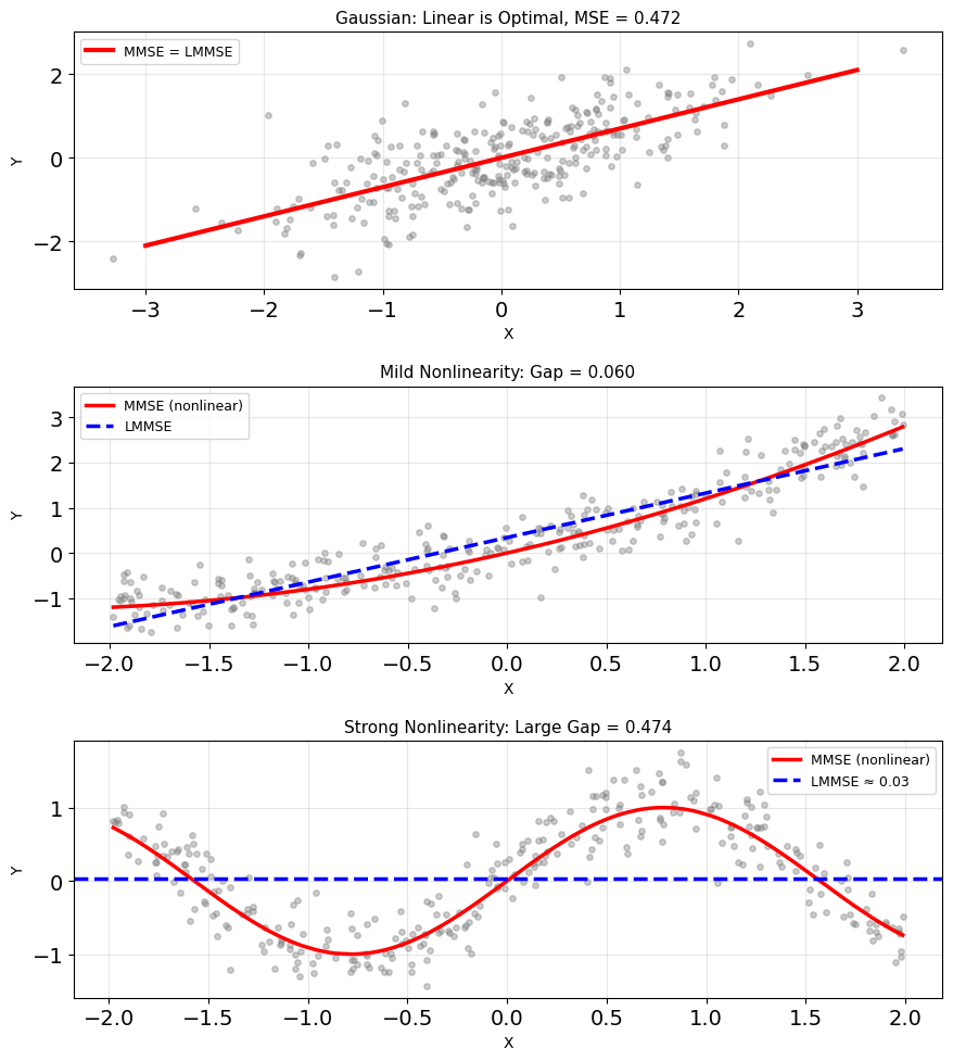
LMMSE = MMSE Iff \(\mathbb{E}[Y|X]\) Is Linear
Restriction can only lose:
\[\text{MSE}_{\text{LMMSE}} \geq \text{MSE}_{\text{MMSE}}\]
Performance gap:
\[\text{MSE}_{\text{LMMSE}} - \text{MSE}_{\text{MMSE}} = \mathbb{E}[(\mathbb{E}[Y|X] - \hat{Y}_{\text{LMMSE}})^2]\]
Measures nonlinearity of \(\mathbb{E}[Y|X]\).
When are they equal?
\[\text{MSE}_{\text{LMMSE}} = \text{MSE}_{\text{MMSE}}\]
if and only if \(\mathbb{E}[Y|X]\) is linear in \(X\).
For jointly Gaussian \((X,Y)\):
- \(\mathbb{E}[Y|X]\) is linear
- LMMSE = MMSE
- No performance loss from restriction
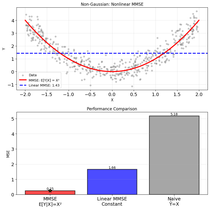
Nonlinear \(\mathbb{E}[Y|X]\) Creates a Performance Gap
Uniform-Quadratic example:
- \(X \sim \text{Uniform}(-2, 2)\)
- \(Y = X^2 + N\), \(N \sim \mathcal{N}(0, 0.5^2)\)
MMSE estimator:
\[\hat{Y}_{\text{MMSE}} = \mathbb{E}[Y|X] = X^2\]
Nonlinear in \(X\)
Linear MMSE (suboptimal): slope \(\text{Cov}(X,Y)/\text{Var}(X) = \mathbb{E}[X^3]/\text{Var}(X) = 0\)
\[\hat{Y}_{\text{linear}} = \mathbb{E}[Y] = \mathbb{E}[X^2] = \frac{4}{3}\]
Performance gap:
- MSE\(_{\text{MMSE}}\) = \(\sigma_N^2\) = 0.25
- MSE\(_{\text{linear}}\) = Var(\(X^2\)) + \(\sigma_N^2 \approx 1.67\)
The gap is Var(\(X^2\)) - the part of \(\mathbb{E}[Y|X]\) no line can follow
Linear Errors Still Carry Nonlinear Structure
MMSE (unrestricted):
\[\mathbb{E}[(Y - \mathbb{E}[Y|X]) \cdot h(X)] = 0 \quad \text{for all } h\]
LMMSE (restricted):
\[\mathbb{E}[(Y - \hat{Y}_{\text{LMMSE}}) \cdot h(X)] = 0 \quad \text{for } h \in \{1, X\}\]
LMMSE error may still correlate with \(X^2, X^3, \sin(X), ...\)
\[\mathbb{E}[(Y - \hat{Y}_{\text{LMMSE}}) \cdot X^2] \neq 0 \text{ (in general)}\]
This correlation is unexploited information—structure in \((X, Y)\) that linear predictors cannot capture.
When LMMSE achieves MMSE:
If \(\mathbb{E}[Y|X]\) is already linear in \(X\):
- LMMSE error \(\perp\) all \(h(X)\) automatically
- No nonlinear structure to exploit
- Gaussian \((X,Y)\) guarantees this
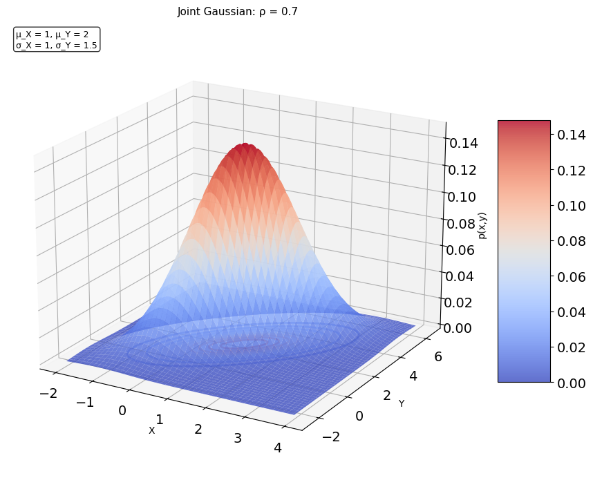
Moments Fully Specify the Bivariate Gaussian
Bivariate Gaussian \((X, Y) \sim \mathcal{N}(\mu, K)\)
Parameters:
\[\mu = \begin{bmatrix} \mu_X \\ \mu_Y \end{bmatrix}, \quad K = \begin{bmatrix} \sigma_X^2 & k_{XY} \\ k_{XY} & \sigma_Y^2 \end{bmatrix}\]
where \(k_{XY} = \rho\sigma_X\sigma_Y\)
Joint density:
\[p(x,y) = \frac{1}{2\pi\sigma_X\sigma_Y\sqrt{1-\rho^2}} \exp\left(-\frac{1}{2(1-\rho^2)}\left[z_x^2 - 2\rho z_x z_y + z_y^2\right]\right)\]
where \(z_x = \frac{x-\mu_X}{\sigma_X}\) and \(z_y = \frac{y-\mu_Y}{\sigma_Y}\) are standardized variables
Fully determined by first and second moments
- 5 parameters: \(\mu_X, \mu_Y, \sigma_X^2, \sigma_Y^2, \rho\)
- All higher moments determined by these
Gaussian \(Y|X\) Has Linear Mean, Constant Variance
Result: \(Y|X=x\) is Gaussian
Conditional mean:
\[\mathbb{E}[Y|X=x] = \mu_Y + \rho\frac{\sigma_Y}{\sigma_X}(x - \mu_X)\]
Conditional variance (constant):
\[\text{Var}(Y|X=x) = \sigma_Y^2(1 - \rho^2)\]
Therefore:
\[Y|X=x \sim \mathcal{N}\left(\mu_Y + \rho\frac{\sigma_Y}{\sigma_X}(x - \mu_X), \sigma_Y^2(1 - \rho^2)\right)\]
Observations:
- \(\mathbb{E}[Y|X=x]\) is linear in \(x\)
- \(\text{Var}(Y|X=x)\) does not depend on \(x\)
- Conditional distribution is still Gaussian
Endpoints:
- \(\rho = 0\): \(\mathbb{E}[Y|X=x] = \mu_Y\) - no information from observation
- \(|\rho| = 1\): \(\text{Var}(Y|X) = 0\) - perfect prediction
Regression line:
\[y = \mu_Y + \rho\frac{\sigma_Y}{\sigma_X}(x - \mu_X)\]
passes through \((\mu_X, \mu_Y)\) with slope \(\rho\sigma_Y/\sigma_X\)
Three Methods Give the Same Linear Formula
Method 1: Complete the square
Start with joint density, condition on \(X = x\):
\[p(y|x) \propto \exp\left(-\frac{1}{2(1-\rho^2)\sigma_Y^2}\left(y - \mu_Y - \rho\frac{\sigma_Y}{\sigma_X}(x-\mu_X)\right)^2\right)\]
Method 2: Linear projection
Find \(a, b\) minimizing \(\mathbb{E}[(Y - aX - b)^2]\):
- \(a^* = \text{Cov}(X,Y)/\text{Var}(X) = \rho\sigma_Y/\sigma_X\)
- \(b^* = \mathbb{E}[Y] - a^*\mathbb{E}[X] = \mu_Y - a^*\mu_X\)
Method 3: Schur complement
Using block matrix operations on \(K\):
\[\mathbb{E}[Y|X=x] = \mu_Y + k_{YX}k_{XX}^{-1}(x - \mu_X)\]
\[= \mu_Y + \rho\sigma_X\sigma_Y \cdot \frac{1}{\sigma_X^2}(x - \mu_X)\]
(all methods give same result)
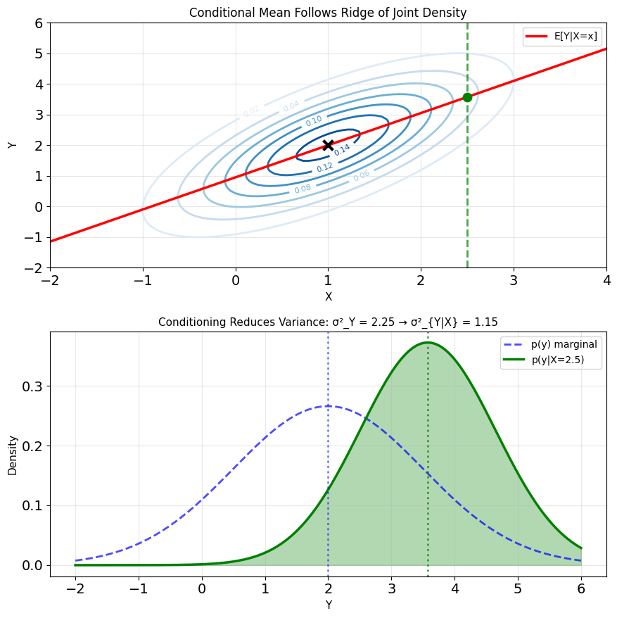
MMSE = LMMSE for Gaussian
For jointly Gaussian \((X, Y)\):
\[\boxed{\hat{Y}_{\text{MMSE}} = \hat{Y}_{\text{LMMSE}} = \mu_Y + \rho\frac{\sigma_Y}{\sigma_X}(X - \mu_X)}\]
Why equal?
- MMSE: \(\hat{Y}_{\text{MMSE}} = \mathbb{E}[Y|X]\)
- For Gaussian: \(\mathbb{E}[Y|X]\) is linear
- LMMSE: Best linear predictor
Minimum MSE:
\[\text{MSE}_{\min} = \sigma_Y^2(1 - \rho^2)\]
Implications:
- No need to consider nonlinear predictors
- Second moments sufficient for optimal prediction
- Closed-form solution
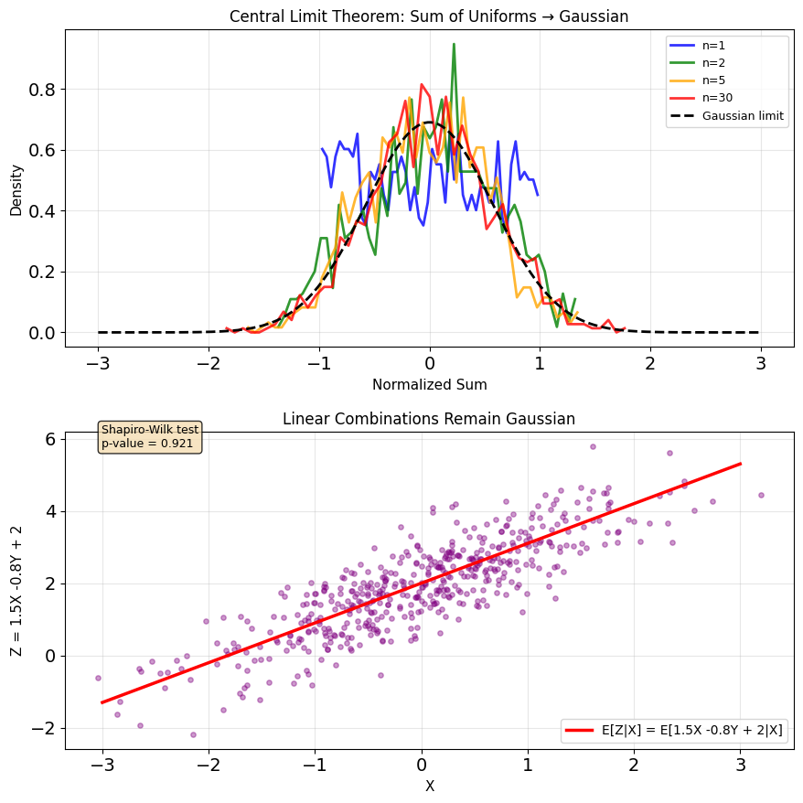
CLT and Max Entropy Justify Gaussian Models
Maximum entropy property: Among all distributions with given mean and covariance, Gaussian has maximum entropy
\[H(X,Y) = -\int\int p(x,y)\log p(x,y) \, dx \, dy\]
Central Limit Theorem: Sum of many independent effects \(\to\) Gaussian
\[\frac{1}{\sqrt{n}}\sum_{i=1}^n (X_i - \mu) \xrightarrow{d} \mathcal{N}(0, \sigma^2)\]
Preserved under linear operations: If \((X,Y)\) Gaussian and \(Z = aX + bY + c\):
- \(Z\) is Gaussian
- \((X,Z)\) jointly Gaussian
- \((Y,Z)\) jointly Gaussian
Sufficient statistics: For Gaussian, sample mean and covariance are sufficient
- No information lost by summarizing with \((\bar{X}, \bar{Y}, S_{XX}, S_{YY}, S_{XY})\)
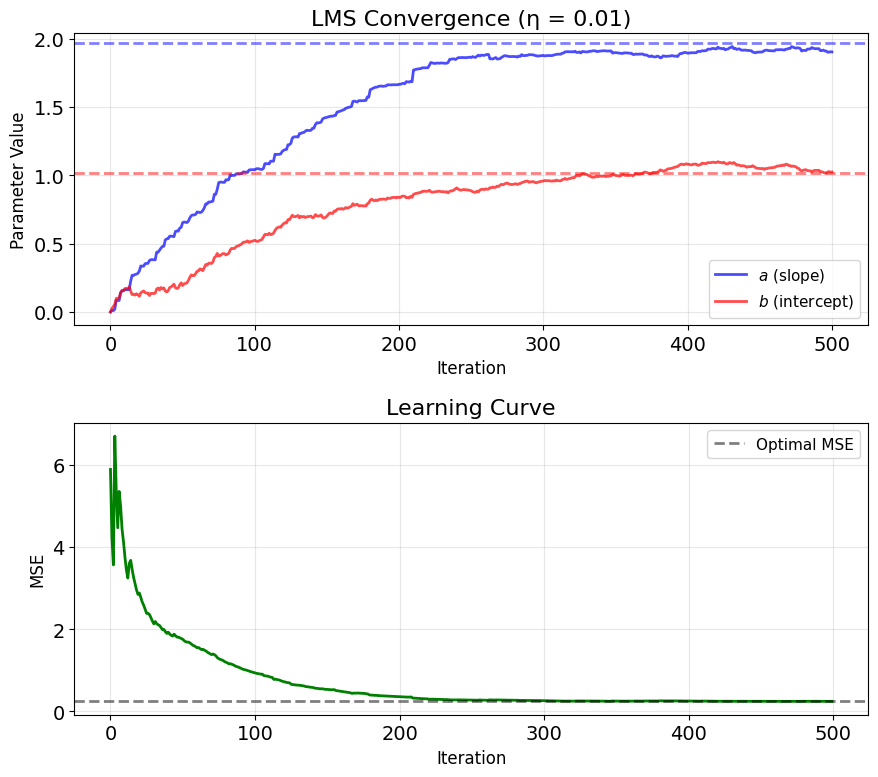
LMS Learns LMMSE from Streaming Data
Problem: the statistics are unknown
LMMSE needs: \(\text{Cov}(X,Y)\) and \(\text{Var}(X)\)
Solution: Learn from streaming data
Population gradient:
\[\frac{\partial}{\partial a} \mathbb{E}[(Y - aX - b)^2] = -2\mathbb{E}[(Y - aX - b)X]\]
Widrow-Hoff: replace the expectation with its one-sample estimate
\[\mathbb{E}[(Y - aX - b)X] \approx (y_i - ax_i - b)x_i = e_i x_i\]
\(x_i y_i\), \(x_i^2\): rank-one instantaneous estimates of \(\mathbb{E}[XY]\), \(\mathbb{E}[X^2]\)
LMS update rule:
\[a_{i+1} = a_i + \eta e_i x_i\]
\[b_{i+1} = b_i + \eta e_i\]
where \(e_i = y_i - \hat{y}_i\) is prediction error and \(\eta\) the step size (sometimes write \(\mu\))
Convergence: \(a_i \to a^*_{\text{LMMSE}}\) as \(i \to \infty\)
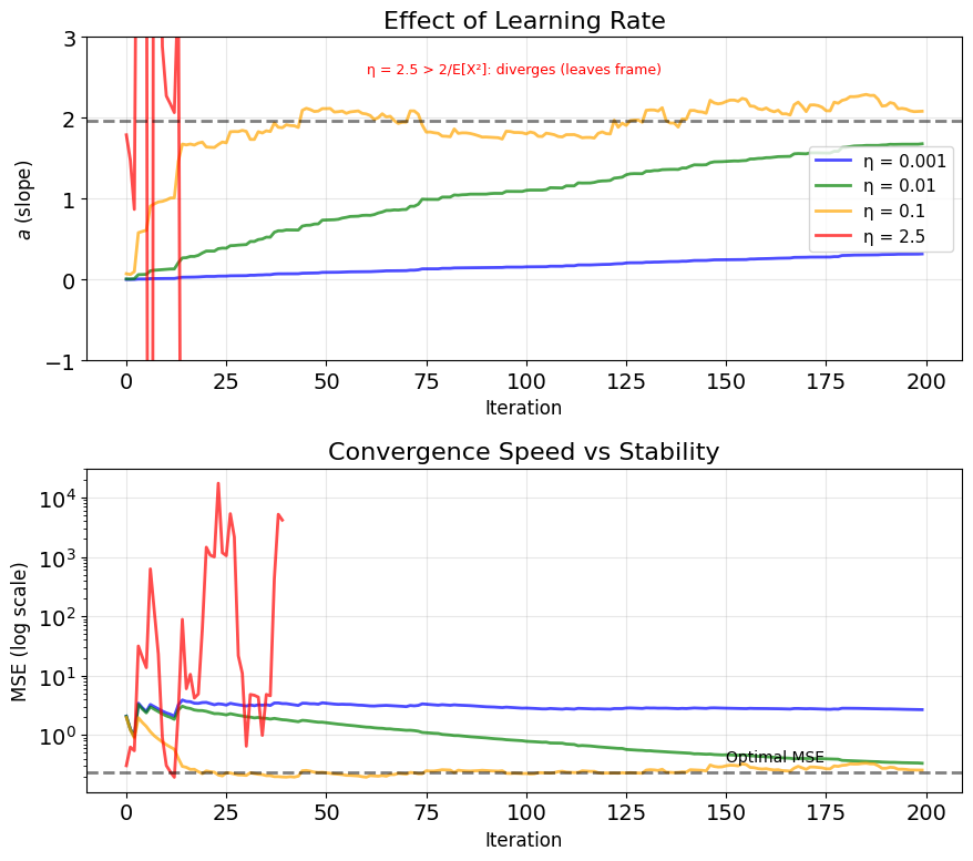
Learning Rate Trades Convergence for Variance
Convergence condition (in the mean):
\[0 < \eta < \frac{2}{\mathbb{E}[X^2]}\]
Too large \(\eta\) \(\Rightarrow\) divergence
Steady-state error:
Misadjustment (small \(\eta\)): \(M = \frac{\eta \mathbb{E}[X^2]}{2}\)
Trade-off:
- Small \(\eta\): Slow convergence, low steady-state error
- Large \(\eta\): Fast convergence, high steady-state error
Time constant:
\[\tau \approx \frac{1}{2\eta \mathbb{E}[X^2]}\]
iterations to converge
Advantages:
- No matrix operations
- Adapts to changing statistics
- Simple hardware implementation
Relation: LMS = stochastic gradient descent for MSE
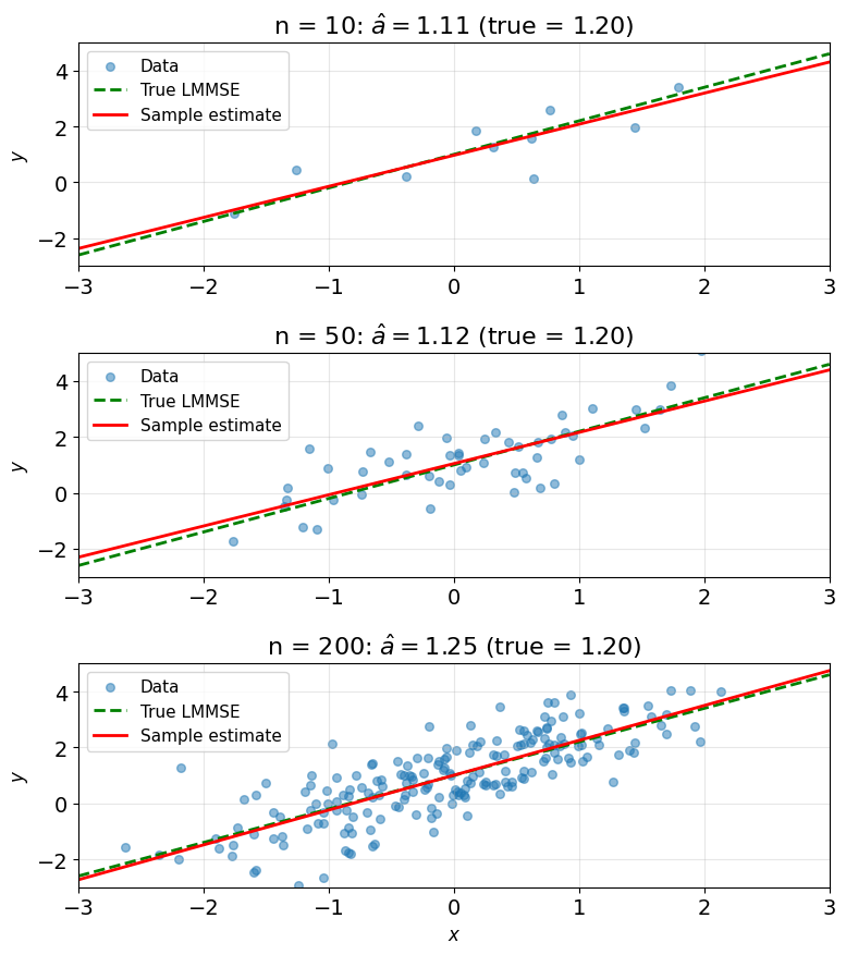
Sample LMMSE Converges to Population LMMSE
Theory (Population)
Given joint distribution \(p(x,y)\):
\[\text{MSE} = \mathbb{E}[(Y - \hat{Y})^2]\]
Linear MMSE solution:
\[a^* = \frac{\text{Cov}(X,Y)}{\text{Var}(X)} = \frac{\mathbb{E}[XY] - \mathbb{E}[X]\mathbb{E}[Y]}{\mathbb{E}[X^2] - \mathbb{E}[X]^2}\]
Practice (Sample)
Given data \(\{(x_i, y_i)\}_{i=1}^n\):
\[\text{MSE}_n = \frac{1}{n}\sum_{i=1}^n (y_i - \hat{y}_i)^2\]
Sample estimates:
\[\hat{a} = \frac{\sum_i (x_i - \bar{x})(y_i - \bar{y})}{\sum_i (x_i - \bar{x})^2}\]
Convergence: \(\hat{a} \to a^*\) as \(n \to \infty\) (law of large numbers)
This is linear regression
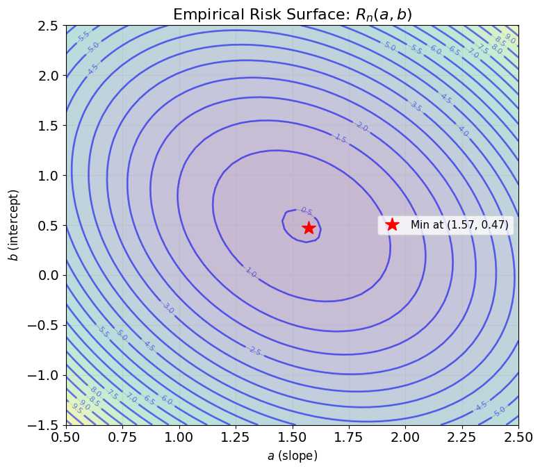
Minimizing Sample MSE = Least Squares
Population risk (unknown):
\[R(a,b) = \mathbb{E}[(Y - aX - b)^2]\]
Empirical risk (computable):
\[R_n(a,b) = \frac{1}{n}\sum_{i=1}^n (y_i - ax_i - b)^2\]
Optimization:
\[\frac{\partial R_n}{\partial b} = -\frac{2}{n}\sum_{i=1}^n (y_i - ax_i - b) = 0\]
\[\implies b = \bar{y} - a\bar{x}\]
\[\frac{\partial R_n}{\partial a} = -\frac{2}{n}\sum_{i=1}^n x_i(y_i - ax_i - b) = 0\]
\[\implies a = \frac{\sum_i x_i y_i - n\bar{x}\bar{y}}{\sum_i x_i^2 - n\bar{x}^2}\]
Sample optimization gives sample LMMSE
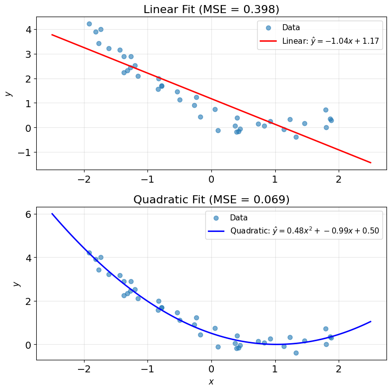
Feature Maps Allow Nonlinear Fits
Linear model limitations:
\[\hat{y} = ax + b\]
Can only model linear relationships
Feature transformation:
\[\hat{y} = \sum_{k=0}^{K} w_k \phi_k(x) = \mathbf{w}^T \boldsymbol{\phi}(x)\]
where \(\boldsymbol{\phi}(x) = [\phi_0(x), \phi_1(x), ..., \phi_K(x)]^T\)
Still linear MMSE in feature space:
- Design matrix: \(\Phi_{ij} = \phi_j(x_i)\)
- Solution: \(\mathbf{w}^* = (\Phi^T\Phi)^{-1}\Phi^T\mathbf{y}\)
Example: Polynomial features
\[\phi_0(x) = 1, \quad \phi_1(x) = x, \quad \phi_2(x) = x^2\]
Now can fit parabolas while still using linear methods
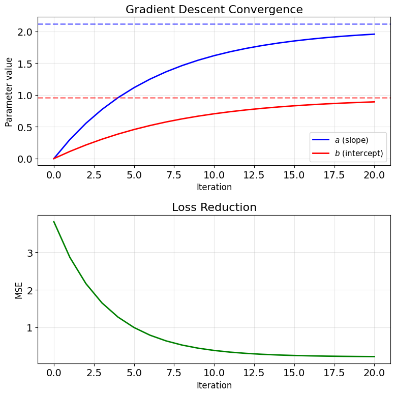
Gradient Descent Recovers LMMSE Iteratively
Batch gradient descent:
\[J(a,b) = \frac{1}{n}\sum_{i=1}^n (y_i - ax_i - b)^2\]
Gradients:
\[\frac{\partial J}{\partial a} = -\frac{2}{n}\sum_{i=1}^n x_i(y_i - ax_i - b)\]
\[\frac{\partial J}{\partial b} = -\frac{2}{n}\sum_{i=1}^n (y_i - ax_i - b)\]
Update:
\[a_{t+1} = a_t - \eta \frac{\partial J}{\partial a}\]
\[b_{t+1} = b_t - \eta \frac{\partial J}{\partial b}\]
One sample per step recovers LMS: the single-sample gradient step is exactly the LMS update; minibatches interpolate between the two
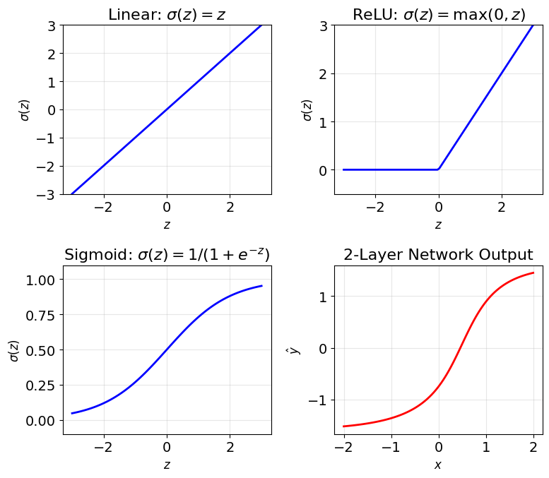
Neural Networks Compose Linear Maps + Nonlinearities
LMMSE \(\neq\) MMSE when \(\mathbb{E}[Y|X]\) is nonlinear.
Single neuron:
\[z = \mathbf{w}^T\mathbf{x} + b\]
\[h = \sigma(z)\]
where \(\sigma\) is activation (ReLU, sigmoid, etc.)
Without activation: Linear regression
\[\hat{y} = \mathbf{w}^T\mathbf{x} + b\]
With activation: Nonlinear transform
\[\hat{y} = \sigma(\mathbf{w}^T\mathbf{x} + b)\]
Deep network: Composition of layers
\[\mathbf{h}^{(1)} = \sigma(\mathbf{W}^{(1)}\mathbf{x} + \mathbf{b}^{(1)})\]
\[\mathbf{h}^{(2)} = \sigma(\mathbf{W}^{(2)}\mathbf{h}^{(1)} + \mathbf{b}^{(2)})\]
\[\hat{y} = \mathbf{W}^{(L)}\mathbf{h}^{(L-1)} + b^{(L)}\]
Objective: \(\frac{1}{n}\sum_i (y_i - \hat{y}_i)^2\) (same MSE)
Backpropagation: Chain rule for gradients
Covariance Matrices Encode Pairwise Relationships
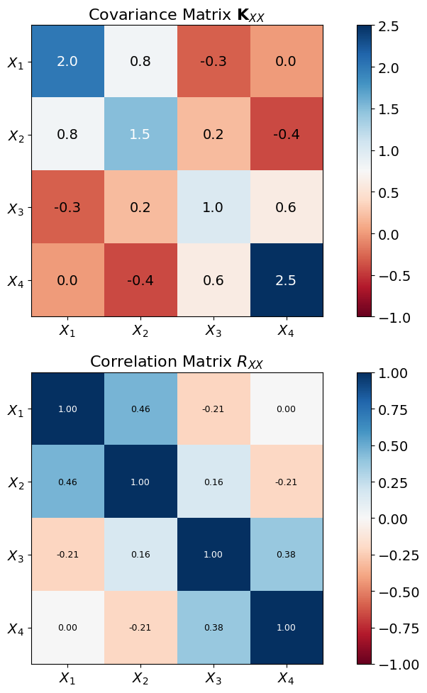
Random vector: \(\mathbf{X} = [X_1, X_2, ..., X_p]^T\)
Mean vector:
\[\boldsymbol{\mu} = \mathbb{E}[\mathbf{X}] = \begin{bmatrix} \mathbb{E}[X_1] \\ \mathbb{E}[X_2] \\ \vdots \\ \mathbb{E}[X_p] \end{bmatrix}\]
Covariance matrix:
\[\mathbf{K}_{XX} = \mathbb{E}[(\mathbf{X} - \boldsymbol{\mu})(\mathbf{X} - \boldsymbol{\mu})^T]\]
Element structure:
\[[\mathbf{K}_{XX}]_{ij} = \text{Cov}(X_i, X_j) = \mathbb{E}[(X_i - \mu_i)(X_j - \mu_j)]\]
Properties:
- Symmetric: \(\mathbf{K}_{XX} = \mathbf{K}_{XX}^T\)
- Positive semi-definite: \(\mathbf{a}^T \mathbf{K}_{XX} \mathbf{a} \geq 0\)
- Diagonal elements = variances
- Off-diagonal = covariances
Positive Definite Matrices Give Rise to Ellipsoids
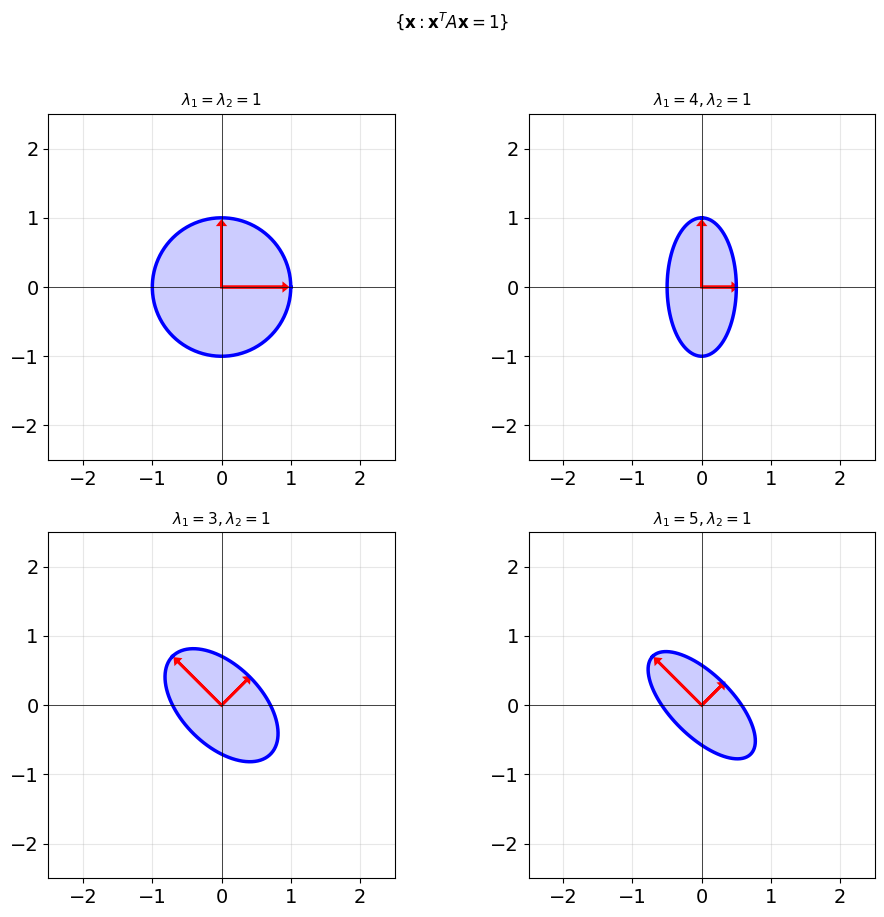
Definition: \(\mathbf{A}\) is positive definite if
\[\mathbf{x}^T \mathbf{A} \mathbf{x} > 0 \quad \text{for all } \mathbf{x} \neq \mathbf{0}\]
Equivalent conditions:
- All eigenvalues \(\lambda_i > 0\)
- \(\mathbf{A} = \mathbf{B}^T\mathbf{B}\) for some invertible \(\mathbf{B}\)
- All leading principal minors positive
Geometric interpretation:
The set \(\{\mathbf{x} : \mathbf{x}^T \mathbf{A} \mathbf{x} = 1\}\) is an ellipsoid.
- Principal axes: eigenvectors of \(\mathbf{A}\)
- Axis lengths: \(1/\sqrt{\lambda_i}\)
Covariance ellipse: for Gaussian data, \((\mathbf{x} - \boldsymbol{\mu})^T \mathbf{K}_{XX}^{-1} (\mathbf{x} - \boldsymbol{\mu}) = c^2\) contains about 95% of the data at \(c \approx 2.45\) - the shape of a data cloud is its covariance
Multiple Predictors Enter Through a Weight Vector
Scalar case:
\[\hat{Y} = aX + b\]
Given: \(X\) (single predictor), predict \(Y\)
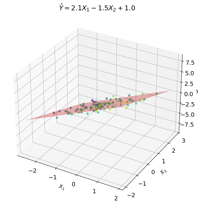
Vector case:
\[\hat{Y} = \mathbf{a}^T\mathbf{X} + b\]
Given: \(\mathbf{X} = [X_1, X_2, ..., X_p]^T\) (multiple predictors)
Example: Predict temperature \(Y\) from:
- \(X_1\) = humidity sensor
- \(X_2\) = pressure sensor
- \(X_3\) = wind speed
Matrix notation:
\[\hat{Y} = \mathbf{a}^T\mathbf{X} + b = \sum_{j=1}^p a_j X_j + b\]
where \(\mathbf{a} = [a_1, a_2, ..., a_p]^T\) are weights
Vector LMMSE Minimizes a Quadratic in \(\mathbf{a}\)
Minimize MSE over linear predictors:
\[\text{MSE}(\mathbf{a}, b) = \mathbb{E}[(Y - \mathbf{a}^T\mathbf{X} - b)^2]\]
Taking derivatives:
\[\frac{\partial \text{MSE}}{\partial b} = -2\mathbb{E}[Y - \mathbf{a}^T\mathbf{X} - b] = 0\]
\[\implies b = \mathbb{E}[Y] - \mathbf{a}^T\mathbb{E}[\mathbf{X}]\]
\[\frac{\partial \text{MSE}}{\partial \mathbf{a}} = -2\mathbb{E}[\mathbf{X}(Y - \mathbf{a}^T\mathbf{X} - b)] = \mathbf{0}\]
Substituting \(b\) and simplifying:
\[\left(\mathbb{E}[\mathbf{X}\mathbf{X}^T] - \mathbb{E}[\mathbf{X}]\mathbb{E}[\mathbf{X}]^T\right)\mathbf{a} = \mathbb{E}[\mathbf{X}Y] - \mathbb{E}[\mathbf{X}]\mathbb{E}[Y]\]
Define:
- \(\mathbf{K}_{XX} = \mathbb{E}[\mathbf{X}\mathbf{X}^T] - \mathbb{E}[\mathbf{X}]\mathbb{E}[\mathbf{X}]^T\) (covariance matrix)
- \(\mathbf{k}_{XY} = \mathbb{E}[\mathbf{X}Y] - \mathbb{E}[\mathbf{X}]\mathbb{E}[Y]\) (cross-covariance vector)
Reminder (vector derivatives, \(\mathbf{A}\) symmetric):
\[\frac{\partial}{\partial \mathbf{a}}\, \mathbf{a}^T\mathbf{x} = \mathbf{x} \qquad\qquad \frac{\partial}{\partial \mathbf{a}}\, \mathbf{a}^T\mathbf{A}\mathbf{a} = 2\mathbf{A}\mathbf{a}\]
\[\frac{\partial}{\partial \mathbf{a}}\, (c - \mathbf{a}^T\mathbf{x})^2 = -2(c - \mathbf{a}^T\mathbf{x})\,\mathbf{x}\]
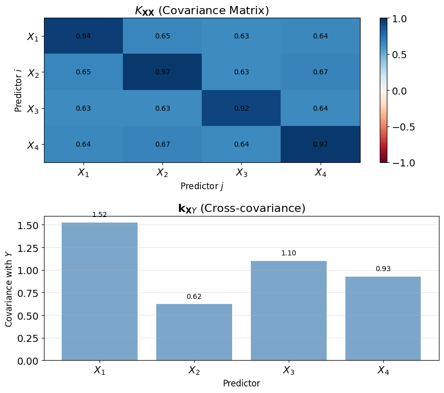
Normal Equations: \(\mathbf{K}_{XX} \mathbf{a} = \mathbf{k}_{XY}\)
Normal equations:
\[\mathbf{K}_{XX}\mathbf{a} = \mathbf{k}_{XY}\]
Solution (if \(\mathbf{K}_{XX}\) invertible):
\[\mathbf{a}^* = \mathbf{K}_{XX}^{-1}\mathbf{k}_{XY}\]
\[b^* = \mathbb{E}[Y] - (\mathbf{a}^*)^T\mathbb{E}[\mathbf{X}]\]
LMMSE predictor:
\[\hat{Y}_{\text{LMMSE}} = \mathbb{E}[Y] + (\mathbf{a}^*)^T(\mathbf{X} - \mathbb{E}[\mathbf{X}])\]
Minimum MSE:
\[\text{MSE}_{\min} = \text{Var}(Y) - \mathbf{k}_{XY}^T \mathbf{K}_{XX}^{-1} \mathbf{k}_{XY}\]
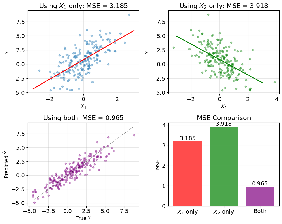
Variance reduction = \(\mathbf{k}_{XY}^T \mathbf{K}_{XX}^{-1} \mathbf{k}_{XY} \geq 0\)
- \(\mathbf{K}_{XX}^{-1}\) is positive definite
- Adding predictors never raises the MSE; zero gain only when \(\mathbf{k}_{XY} = \mathbf{0}\)
LMMSE = Projection onto Column Space
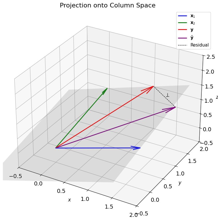
Column space perspective:
Data matrix columns: \(\mathbf{x}_1, \mathbf{x}_2, ..., \mathbf{x}_p\)
\[\mathcal{S} = \text{span}(\mathbf{x}_1, \mathbf{x}_2, ..., \mathbf{x}_p)\]
LMMSE = Projection:
\[\hat{\mathbf{y}} = \text{Proj}_{\mathcal{S}}(\mathbf{y})\]
Orthogonality:
\[\mathbf{y} - \hat{\mathbf{y}} \perp \mathcal{S}\]
Equivalently: \(\mathbf{X}^T(\mathbf{y} - \mathbf{X}\mathbf{a}) = \mathbf{0}\) - the normal equations in sample form, \(\mathbf{X}^T\mathbf{X}\mathbf{a} = \mathbf{X}^T\mathbf{y}\)
Projection matrix:
\[\mathbf{P} = \mathbf{X}(\mathbf{X}^T\mathbf{X})^{-1}\mathbf{X}^T\]
\[\hat{\mathbf{y}} = \mathbf{P}\mathbf{y}\]
Properties:
- \(\mathbf{P}^2 = \mathbf{P}\) (idempotent)
- \(\mathbf{P}^T = \mathbf{P}\) (symmetric)
- \(\text{rank}(\mathbf{P}) = p\) (dimension of \(\mathcal{S}\))
Gaussian Vectors Are Closed Under Linear Transforms
Joint Gaussian distribution:
\(\begin{bmatrix} \mathbf{X} \\ \mathbf{Y} \end{bmatrix} \sim \mathcal{N}\left(\begin{bmatrix} \boldsymbol{\mu}_X \\ \boldsymbol{\mu}_Y \end{bmatrix}, \begin{bmatrix} \mathbf{K}_{XX} & \mathbf{K}_{XY} \\ \mathbf{K}_{YX} & \mathbf{K}_{YY} \end{bmatrix}\right)\)
Probability density:
\[p(\mathbf{x}, \mathbf{y}) = \frac{1}{(2\pi)^{(p+m)/2}|\mathbf{K}|^{1/2}} \exp\left(-\frac{1}{2}\mathbf{z}^T\mathbf{K}^{-1}\mathbf{z}\right)\]
where \(\mathbf{z} = \begin{bmatrix} \mathbf{x} - \boldsymbol{\mu}_X \\ \mathbf{y} - \boldsymbol{\mu}_Y \end{bmatrix}\)
Linear operations preserve Gaussianity
If \(\mathbf{Z} = \mathbf{A}\mathbf{X} + \mathbf{b}\), then:
\[\mathbf{Z} \sim \mathcal{N}(\mathbf{A}\boldsymbol{\mu}_X + \mathbf{b}, \mathbf{A}\mathbf{K}_{XX}\mathbf{A}^T)\]
Marginals are Gaussian:
\[\mathbf{X} \sim \mathcal{N}(\boldsymbol{\mu}_X, \mathbf{K}_{XX})\]
Gaussian Vectors Make Vector LMMSE Optimal
Given joint Gaussian, conditional is also Gaussian:
\[\mathbf{Y}|\mathbf{X} = \mathbf{x} \sim \mathcal{N}(\boldsymbol{\mu}_{Y|X}, \mathbf{K}_{Y|X})\]
Conditional mean (MMSE estimator):
\[\boldsymbol{\mu}_{Y|X} = \boldsymbol{\mu}_Y + \mathbf{K}_{YX}\mathbf{K}_{XX}^{-1}(\mathbf{x} - \boldsymbol{\mu}_X)\]
Conditional covariance (error covariance):
\[\mathbf{K}_{Y|X} = \mathbf{K}_{YY} - \mathbf{K}_{YX}\mathbf{K}_{XX}^{-1}\mathbf{K}_{XY}\]
The subtracted term is the Schur complement - the uncertainty removed by observing \(\mathbf{X}\)
Observations:
- Conditional mean is linear in \(\mathbf{x}\)
- Conditional covariance does not depend on \(\mathbf{x}\)
- For Gaussian: MMSE = Linear MMSE
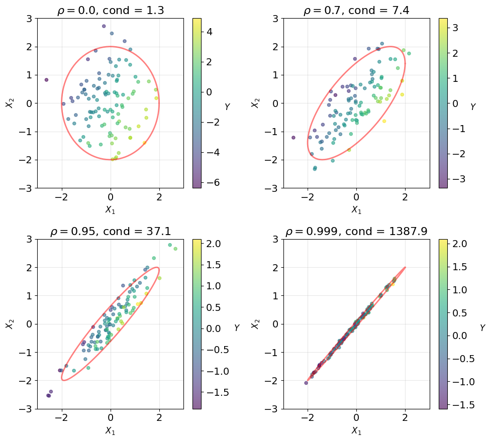
Collinearity Ill-Conditions \(\mathbf{K}_{XX}\)
Direct inversion issues:
-
Ill-conditioning: When predictors highly correlated
- \(\text{cond}(\mathbf{K}_{XX}) = \frac{\lambda_{\max}}{\lambda_{\min}} \gg 1\)
- Small changes \(\to\) large parameter changes
-
Rank deficiency: perfect collinearity, or a sample estimate \(\hat{\mathbf{K}}_{XX}\) with \(p > n\)
- \(\mathbf{K}_{XX}\) not invertible
- Infinitely many solutions
Solutions:
-
QR decomposition: \(\mathbf{X} = \mathbf{Q}\mathbf{R}\)
- More stable than normal equations
- \(\mathbf{a} = \mathbf{R}^{-1}\mathbf{Q}^T\mathbf{y}\)
-
SVD: \(\mathbf{X} = \mathbf{U}\boldsymbol{\Sigma}\mathbf{V}^T\)
- Handles rank-deficient cases
- Pseudoinverse: \(\mathbf{X}^+ = \mathbf{V}\boldsymbol{\Sigma}^+ \mathbf{U}^T\)
-
Regularization:
- Ridge: Add \(\lambda \mathbf{I}\) to \(\mathbf{K}_{XX}\)
- Makes problem well-posed
- Trades bias for stability
Multiple Outputs Decompose into Scalar Problems
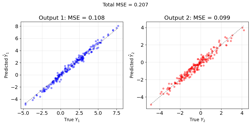
Multiple responses:
\[\mathbf{Y} = [Y_1, Y_2, ..., Y_m]^T\]
Linear model:
\[\hat{\mathbf{Y}} = \mathbf{W}^T\mathbf{X} + \mathbf{b}\]
where \(\mathbf{W} \in \mathbb{R}^{p \times m}\) is the weight matrix
MSE matrix:
\[\mathbf{M} = \mathbb{E}[(\mathbf{Y} - \hat{\mathbf{Y}})(\mathbf{Y} - \hat{\mathbf{Y}})^T]\]
Minimize trace (total MSE):
\[\text{tr}(\mathbf{M}) = \sum_{i=1}^m \mathbb{E}[(Y_i - \hat{Y}_i)^2]\]
Solution:
\[\mathbf{W}^* = \mathbf{K}_{XX}^{-1}\mathbf{K}_{XY}\]
where \(\mathbf{K}_{XY} = \mathbb{E}[\mathbf{X}\mathbf{Y}^T] - \mathbb{E}[\mathbf{X}]\mathbb{E}[\mathbf{Y}]^T\)
Solves as \(m\) separate LMMSE problems - one per output
Eigendecomposition Diagonalizes the Covariance
Computational cost:
When \(\mathbf{K}_{XX}\) has off-diagonal terms:
- Matrix inversion requires \(O(p^3)\) operations
- All variables coupled in solution
- Numerical instability for ill-conditioned matrices
Eigendecomposition approach:
Any symmetric positive semi-definite matrix:
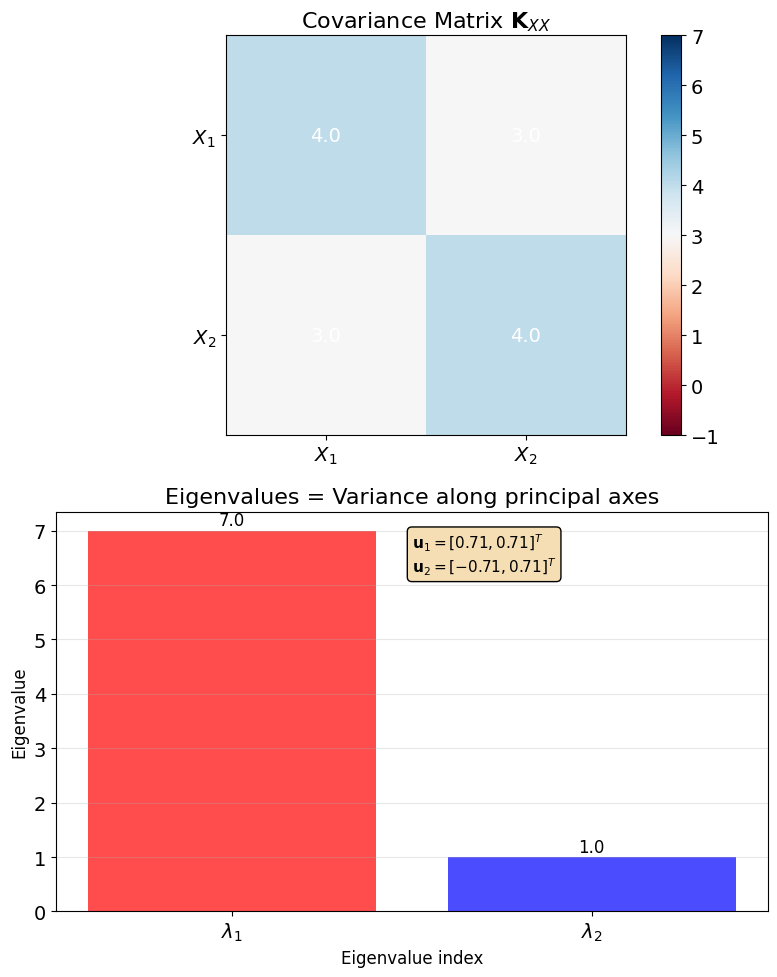
\[\mathbf{K}_{XX} = \mathbf{U}\boldsymbol{\Lambda}\mathbf{U}^T\]
where:
- \(\mathbf{U} = [\mathbf{u}_1, \mathbf{u}_2, ..., \mathbf{u}_p]\) orthonormal
- \(\boldsymbol{\Lambda} = \text{diag}(\lambda_1, \lambda_2, ..., \lambda_p)\)
- \(\lambda_1 \geq \lambda_2 \geq ... \geq \lambda_p \geq 0\)
Eigenvectors are orthogonal
\[\mathbf{u}_i^T \mathbf{u}_j = \delta_{ij}\]
This orthogonality simplifies coordinate transformation.
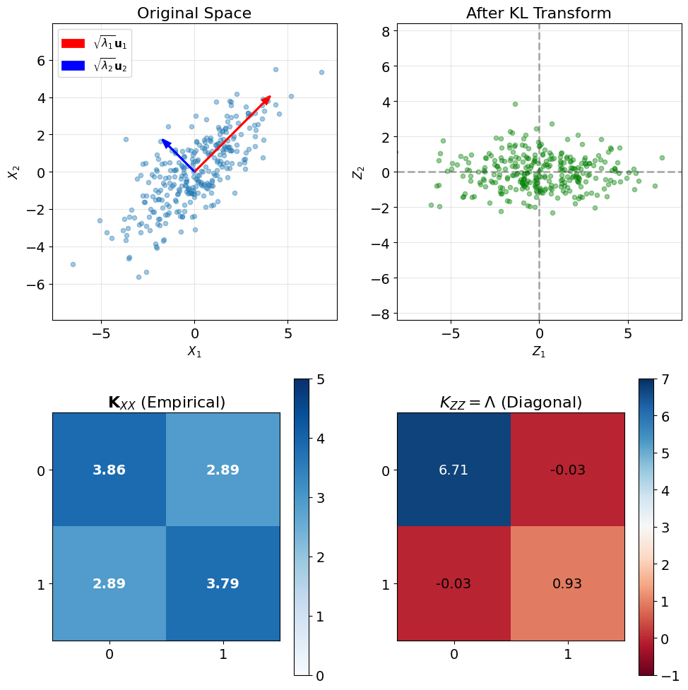
KL Transform Produces Uncorrelated Components
Coordinate transformation:
\[\mathbf{Z} = \mathbf{U}^T\mathbf{X}\]
Covariance in new coordinates:
\[\mathbf{K}_{ZZ} = \mathbb{E}[\mathbf{Z}\mathbf{Z}^T]\]
\[= \mathbb{E}[\mathbf{U}^T\mathbf{X}\mathbf{X}^T\mathbf{U}]\]
\[= \mathbf{U}^T\mathbb{E}[\mathbf{X}\mathbf{X}^T]\mathbf{U}\]
\[= \mathbf{U}^T\mathbf{K}_{XX}\mathbf{U}\]
\[= \mathbf{U}^T(\mathbf{U}\boldsymbol{\Lambda}\mathbf{U}^T)\mathbf{U}\]
\[= \boldsymbol{\Lambda}\]
Result: Diagonal covariance matrix
Components of \(\mathbf{Z}\) are uncorrelated:
\[\mathbb{E}[Z_iZ_j] = \lambda_i\delta_{ij}\]
Inverse transform (reconstruction):
\[\mathbf{X} = \mathbf{U}\mathbf{Z}\]
Since \(\mathbf{U}\) is orthonormal: \(\mathbf{U}^T\mathbf{U} = \mathbf{I}\)
Worked Example: Diagonalizing a \(3 \times 3\) Covariance
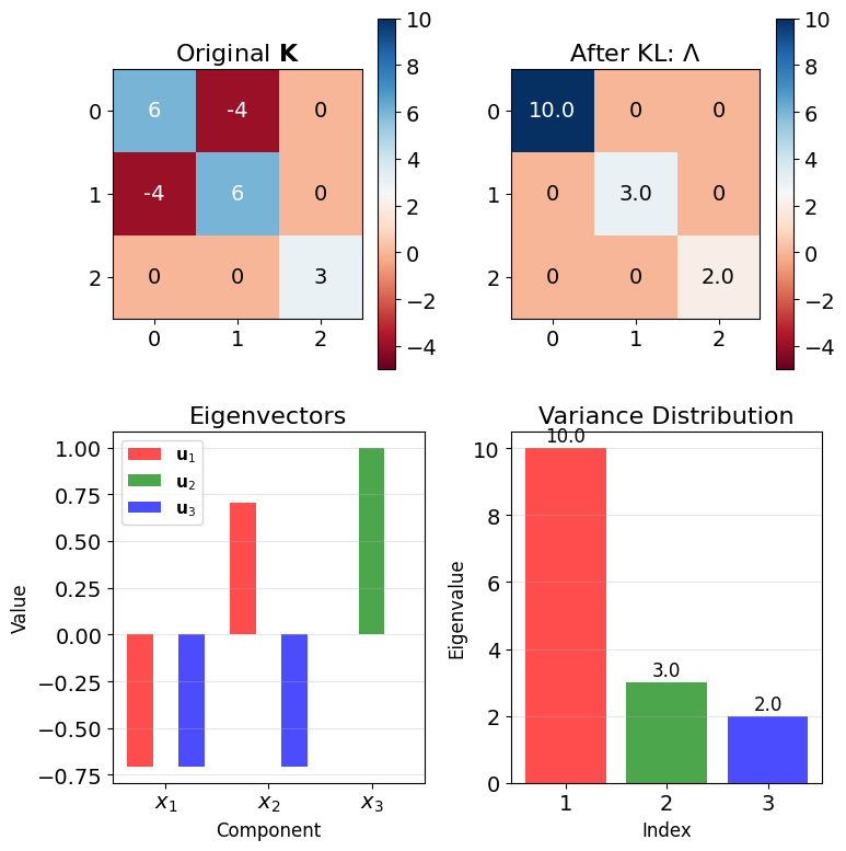
Given covariance:
\[\mathbf{K} = \begin{bmatrix} 6 & -4 & 0 \\ -4 & 6 & 0 \\ 0 & 0 & 3 \end{bmatrix}\]
Find eigenvalues: Solve \(\det(\mathbf{K} - \lambda\mathbf{I}) = 0\)
Block structure simplifies:
- Upper \(2 \times 2\) block: \(\lambda_{1,2} = 6 \pm 4\)
- Lower \(1 \times 1\) block: \(\lambda_3 = 3\)
Result: \(\lambda_1 = 10, \lambda_2 = 3, \lambda_3 = 2\)
Find eigenvectors: Solve \((\mathbf{K} - \lambda_i\mathbf{I})\mathbf{v} = 0\)
\[\mathbf{u}_1 = \frac{1}{\sqrt{2}}\begin{bmatrix}1\\-1\\0\end{bmatrix}, \quad
\mathbf{u}_2 = \begin{bmatrix}0\\0\\1\end{bmatrix}, \quad
\mathbf{u}_3 = \frac{1}{\sqrt{2}}\begin{bmatrix}1\\1\\0\end{bmatrix}\]
Result: \(\mathbf{K}_{ZZ} = \text{diag}(10, 3, 2)\)
Decorrelated Predictors Decouple the Normal Equations
Coupled problem:
\[\mathbf{K}_{XX}\mathbf{a} = \mathbf{k}_{XY}\]
Every component of \(\mathbf{a}\) depends on every entry of \(\mathbf{K}_{XX}\)
In the KL basis \(\mathbf{Z} = \mathbf{U}^T\mathbf{X}\):
\(\mathbf{K}_{ZZ} = \boldsymbol{\Lambda}\), so the normal equations diagonalize:
\[\lambda_i \, a_{z,i} = \text{Cov}(Z_i, Y) \implies a_{z,i} = \frac{\text{Cov}(Z_i, Y)}{\lambda_i}\]
Each coefficient solved independently
Cost: eigendecomposition is \(O(p^3)\), like inversion - the gain is structure, not speed
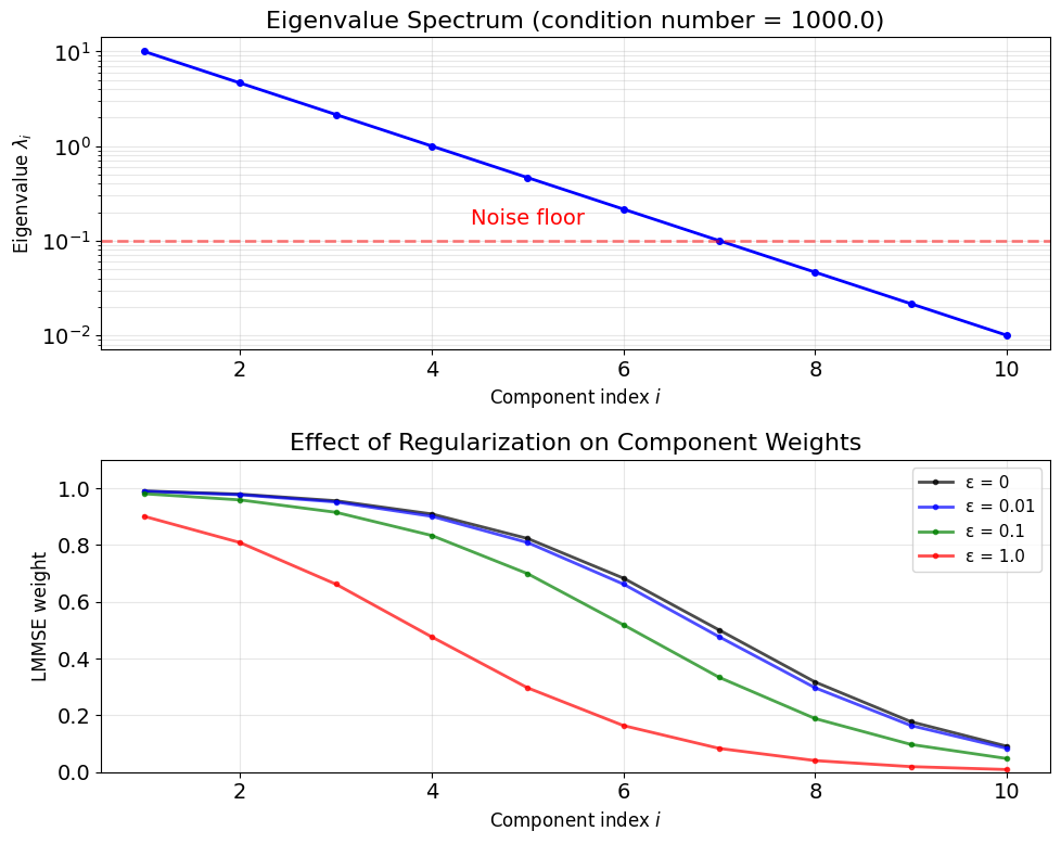
- Conditioning read off the spectrum: small \(\lambda_i\) inflate \(a_{z,i}\)
- Per-component regularization:
\[a_{z,i} = \frac{\text{Cov}(Z_i, Y)}{\lambda_i + \epsilon}\]
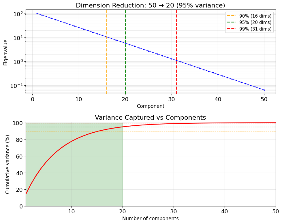
- Truncating small-\(\lambda_i\) components: principal-component regression
Truncating Eigenvalues Trades MSE for Dimensionality
Not all dimensions equally informative
Eigenvalues measure variance (information) per dimension.
Truncated representation: Keep only first \(k < p\) components:
\[\mathbf{X} \approx \sum_{i=1}^k Z_i \mathbf{u}_i\]
Selection criterion: Retain fraction \(\alpha\) of total variance:
\[\frac{\sum_{i=1}^k \lambda_i}{\sum_{i=1}^p \lambda_i} \geq \alpha\]
Common choice: \(\alpha = 0.95\) or \(0.99\)
Reconstruction error:
\[\mathbb{E}[\|\mathbf{X} - \hat{\mathbf{X}}_k\|^2] = \sum_{i=k+1}^p \lambda_i\]
Error equals sum of discarded eigenvalues.
Applications:
- Principal Component Analysis (PCA)
- Data compression
- Denoising (discard noisy dimensions)