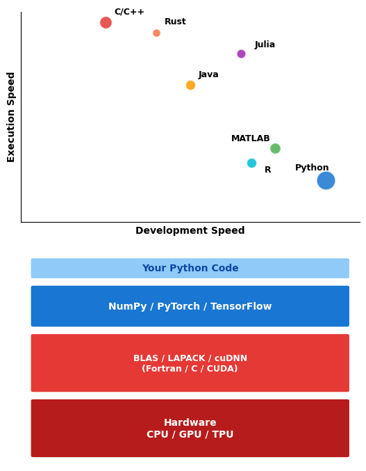
Why Python for Scientific Computing?
A Paradox
Python is 10-100× slower than C/C++ for raw computation, yet dominates scientific computing. Why?
Design Philosophy
- Readability over performance: Code is read more than written
- Dynamic over static: Flexibility for exploration
- Extensive standard library: Reduces external dependencies
- Glue language: Binds fast libraries (NumPy, SciPy use C/Fortran)
The Two-Language Problem
Traditional approach: prototype in MATLAB/Python, rewrite in C++ for production
Python’s approach: Python for control flow, C for computation
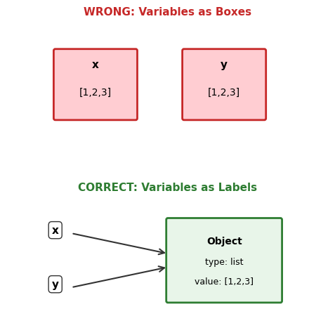
Variables Are Not Boxes
Variables are names bound to objects, not storage locations.
x = [1, 2, 3]  # x refers to a list object
y = x          # y refers to THE SAME object
y.append(4)    # Modifying through y
print(f"x = {x}")  # x sees the change!

# To create a copy:
z = x.copy()   # or x[:] or list(x)
z.append(5)
print(f"x = {x}, z = {z}")  # x unchanged
x = [1, 2, 3, 4]
x = [1, 2, 3, 4], z = [1, 2, 3, 4, 5]
Assignment creates a reference, not a copy.
Immutable types (int, str, tuple): cannot be modified in place—operations create new objects.
Namespace Resolution: The LEGB Rule
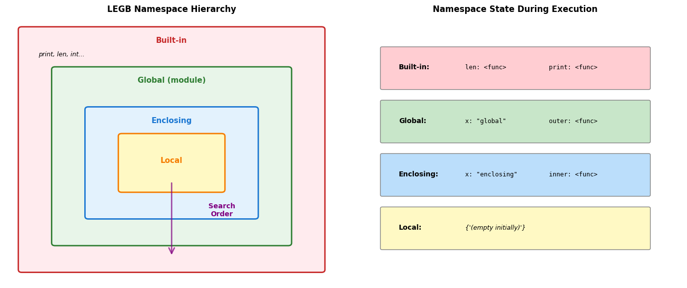
Python resolves names through a hierarchy of namespace dictionaries.
x = "global"  # Global namespace

def outer():
    x = "enclosing"  # Enclosing namespace

    def inner():
        print(f"Reading x: {x}")  # LEGB search finds enclosing

    def inner_local():
        x = "local"  # Creates local binding
        print(f"Local x: {x}")

    inner()
    inner_local()
    print(f"Enclosing x: {x}")

outer()
print(f"Global x: {x}")

# Namespace modification
def show_namespace_dict():
    local_var = 42
    print(f"locals(): {locals()}")
    print(f"'local_var' in locals(): {'local_var' in locals()}")

show_namespace_dict()
Reading x: enclosing
Local x: local
Enclosing x: enclosing
Global x: global
locals(): {'local_var': 42}
'local_var' in locals(): True
Resolution Rules:
- Local: Current function’s namespace
- Enclosing: Outer function(s) namespace
- Global: Module-level namespace
- Built-in: Pre-defined names
Binding Behavior:
- Assignment creates local binding by default
globalkeyword binds to global namespacenonlocalbinds to enclosing namespace- Reading doesn’t create binding
# UnboundLocalError example
count = 0
def increment():
    # Python sees assignment, creates local slot
    # But referenced before assignment
    try:
        count += 1  # UnboundLocalError
    except UnboundLocalError as e:
        print(f"Error: {e}")

increment()
Error: cannot access local variable 'count' where it is not associated with a value
Lists vs Arrays: Memory Layout Matters
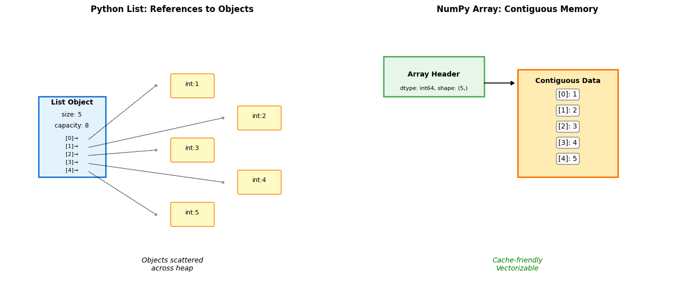
Python lists and NumPy arrays have different memory layouts.
import numpy as np

# Memory comparison
py_list = [1, 2, 3, 4, 5]
np_array = np.array([1, 2, 3, 4, 5])

print(f"Python list overhead: {sys.getsizeof(py_list)} bytes")
print(f"NumPy array overhead: {sys.getsizeof(np_array)} bytes")
print(f"NumPy data buffer: {np_array.nbytes} bytes")

# Performance impact
import timeit
lst = list(range(1000))
arr = np.arange(1000)

t_list = timeit.timeit(lambda: sum(lst), number=10000)
t_numpy = timeit.timeit(lambda: arr.sum(), number=10000)

print(f"\nSum 1000 elements:")
print(f"Python list: {t_list:.4f}s")
print(f"NumPy array: {t_numpy:.4f}s ({t_list/t_numpy:.1f}x faster)")
Python list overhead: 104 bytes
NumPy array overhead: 152 bytes
NumPy data buffer: 40 bytes

Sum 1000 elements:
Python list: 0.0228s
NumPy array: 0.0061s (3.7x faster)
List cost per element:
- 8-byte pointer
- 28-byte int object
- ~36 bytes total per int
NumPy cost:
- ~100-byte header (fixed)
- 8 bytes per element (data only)
Why NumPy wins:
- No pointer chasing
- No per-element type checks
- Single C loop over contiguous memory
- Gap grows with array size
Python’s Execution Model
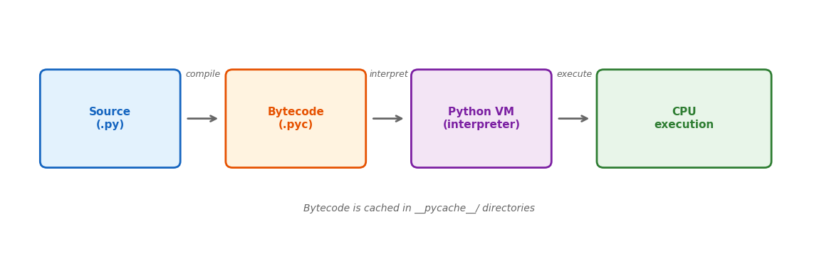
Why this matters:
- No separate compile step — edit and run immediately
- Runtime errors only — syntax errors found when line executes
- Slower than native code — bytecode interpretation has overhead
- Dynamic features — can modify code at runtime (
eval,exec)
Comparison:
| C++ | Java | Python | |
|---|---|---|---|
| Compile to | Machine code | JVM bytecode | PVM bytecode |
| Type checking | Compile time | Compile time | Runtime |
| Speed | Fast | Medium | Slow |
| Edit-run cycle | Slow | Medium | Fast |
Indexing and Slicing
Zero-based indexing. Negative indices count from the end. Slicing creates copies.

Slice syntax: [start:stop:step]
start: First index (inclusive), default 0stop: Last index (exclusive), default lenstep: Increment, default 1
data = [10, 20, 30, 40, 50, 60, 70]

print(f"data[2:5]  = {data[2:5]}")   # [30, 40, 50]
print(f"data[:3]   = {data[:3]}")    # [10, 20, 30]
print(f"data[4:]   = {data[4:]}")    # [50, 60, 70]
print(f"data[::2]  = {data[::2]}")   # [10, 30, 50, 70]
print(f"data[::-1] = {data[::-1]}")  # Reversed
print(f"data[1:-1] = {data[1:-1]}")  # [20, 30, 40, 50, 60]
data[2:5]  = [30, 40, 50]
data[:3]   = [10, 20, 30]
data[4:]   = [50, 60, 70]
data[::2]  = [10, 30, 50, 70]
data[::-1] = [70, 60, 50, 40, 30, 20, 10]
data[1:-1] = [20, 30, 40, 50, 60]
Slicing creates copies (for lists):
original = [1, 2, 3, 4, 5]
copy = original[:]       # Shallow copy
copy[0] = 999
print(f"Original: {original}")
print(f"Copy: {copy}")
Original: [1, 2, 3, 4, 5]
Copy: [999, 2, 3, 4, 5]
Slice assignment (modifies in place):
data = [1, 2, 3, 4, 5]
data[1:4] = [20, 30]     # Replace slice
print(f"After: {data}")

data[2:2] = [100, 200]   # Insert at index 2
print(f"After insert: {data}")
After: [1, 20, 30, 5]
After insert: [1, 20, 100, 200, 30, 5]
Warning: NumPy arrays behave differently — slices are views, not copies.
Sequence Types: Three Design Choices
Python provides three sequence types with different trade-offs.
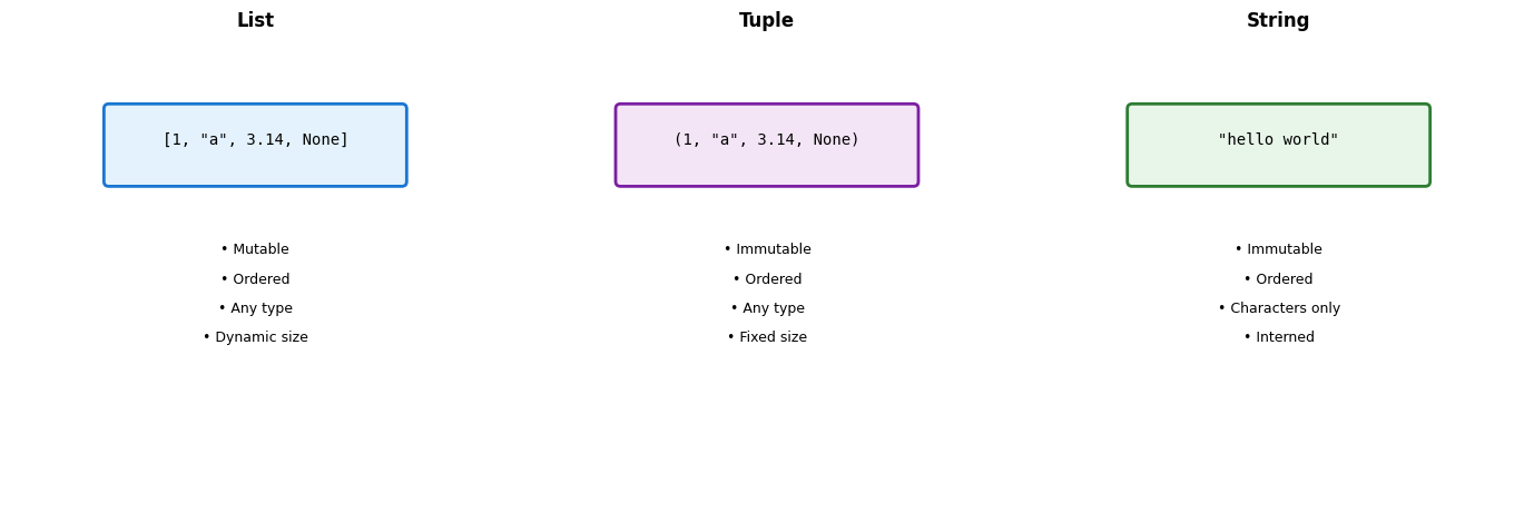
Design Consequences:
- Lists allow heterogeneous data but pay indirection cost
- Tuples trade mutability for hashability and memory efficiency
- Strings optimize for text with specialized methods
import sys

# Memory comparison
lst = [1, 2, 3, 4, 5]
tup = (1, 2, 3, 4, 5)
string = "12345"

print("Memory usage:")
print(f"  List:   {sys.getsizeof(lst)} bytes")
print(f"  Tuple:  {sys.getsizeof(tup)} bytes")
print(f"  String: {sys.getsizeof(string)} bytes")

# Hashability determines dict key eligibility
print("\nCan be dict key:")
for obj, name in [(lst, 'List'), (tup, 'Tuple'), (string, 'String')]:
    try:
        d = {obj: 'value'}
        print(f"  {name}: Yes")
    except TypeError:
        print(f"  {name}: No")
Memory usage:
  List:   104 bytes
  Tuple:  80 bytes
  String: 46 bytes

Can be dict key:
  List: No
  Tuple: Yes
  String: Yes
Big-O Notation: How Cost Scales
Big-O describes how runtime (or memory) grows with input size n, keeping only the dominant term: 3n² + 10n is O(n²).
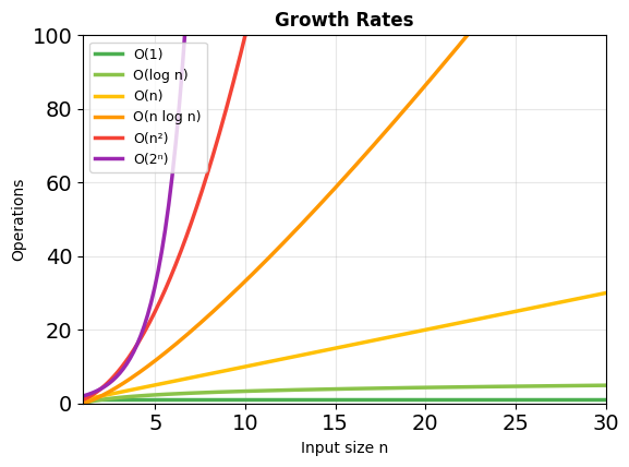
| Class | Name | Python example |
|---|---|---|
| O(1) | Constant | d[key], x in set |
| O(log n) | Logarithmic | binary search (bisect) |
| O(n) | Linear | x in list, sum() |
| O(n log n) | Linearithmic | sorted() |
| O(n²) | Quadratic | nested loops, repeated string += |
| O(2ⁿ) | Exponential | brute force over subsets |
Big-O drops constants. A Python loop and a NumPy C loop are both O(n) but differ ~100× in cost per element. Choose the right growth class first, then the right implementation.
List Internals: Over-allocation Strategy
Lists allocate extra space to amortize the cost of growth.
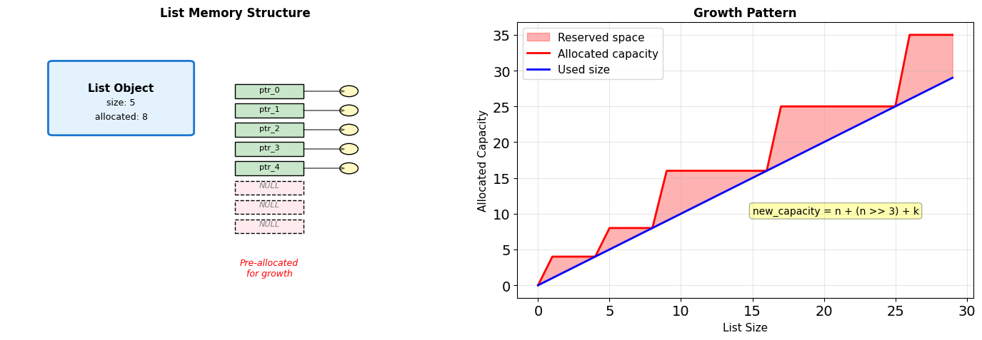
# Observe allocation behavior
import sys

lst = []
sizes_and_caps = []

for i in range(20):
    lst.append(i)
    # Size includes list object overhead
    total_size = sys.getsizeof(lst)
    # Approximate capacity from size
    capacity = (total_size - sys.getsizeof([])) // 8
    sizes_and_caps.append((len(lst), capacity))

# Show growth points
print("Size → Capacity:")
last_cap = 0
for size, cap in sizes_and_caps:
    if cap != last_cap:
        print(f"  {size:2d} → {cap:2d} (grew by {cap - last_cap})")
        last_cap = cap
Size → Capacity:
   1 →  4 (grew by 4)
   5 →  8 (grew by 4)
   9 → 16 (grew by 8)
  17 → 24 (grew by 8)
Growth Strategy:
When a list exceeds capacity, Python:
- Calculates new capacity using formula
- Allocates new pointer array
- Copies all existing pointers
- Frees old array
Cost Analysis:
- Append is O(1) amortized
- Individual append can trigger O(n) reallocation
- Trade memory for performance
List Operations: Implementation Details
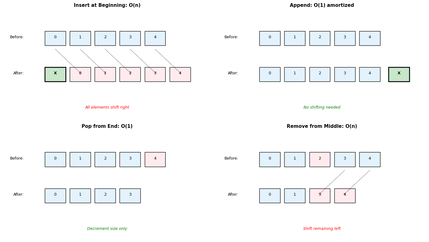
Different operations have different costs based on internal structure.
# Demonstrating operation costs
import time

def measure_operation(lst, operation, description):
    """Measure single operation time."""
    start = time.perf_counter()
    operation(lst)
    elapsed = time.perf_counter() - start
    return elapsed * 1e6  # Convert to microseconds

# Large list for measurable times
n = 100000
test_list = list(range(n))

# Operations
times = {}
times['append'] = measure_operation(test_list.copy(),
                                   lambda l: l.append(999),
                                   "Append")
times['insert_0'] = measure_operation(test_list.copy(),
                                      lambda l: l.insert(0, 999),
                                      "Insert at 0")
times['pop'] = measure_operation(test_list.copy(),
                                lambda l: l.pop(),
                                "Pop from end")
times['pop_0'] = measure_operation(test_list.copy(),
                                   lambda l: l.pop(0),
                                   "Pop from start")

print(f"Operation times (n={n}):")
for op, time in times.items():
    print(f"  {op:12s}: {time:8.2f} μs")
Operation times (n=100000):
  append      :     0.67 μs
  insert_0    :    13.54 μs
  pop         :     0.29 μs
  pop_0       :    11.21 μs
Dictionary Architecture: Open Addressing Hash Table
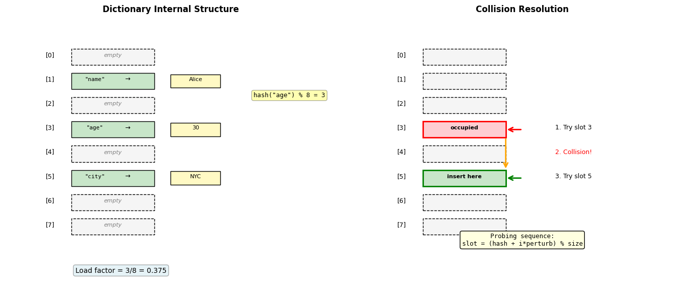
Dictionaries use open addressing with random probing for collision resolution.
# Dictionary internals
d = {'a': 1, 'b': 2, 'c': 3}

# Show hash values
for key in d:
    print(f"hash('{key}') = {hash(key):20d}")

# Dictionary growth
import sys
sizes = []
for i in range(20):
    d = {str(j): j for j in range(i)}
    sizes.append((i, sys.getsizeof(d)))

print("\nDict size growth:")
last_size = 0
for n, size in sizes:
    if size != last_size:
        print(f"  {n:2d} items: {size:4d} bytes")
        last_size = size
hash('a') = -7315216989034702776
hash('b') =  2805302887546029812
hash('c') =  4965872525638186726

Dict size growth:
   0 items:   64 bytes
   1 items:  184 bytes
   6 items:  272 bytes
  11 items:  464 bytes
Design Choices:
- Open addressing: No separate chains, better cache locality
- 2/3 load factor: Resize when 2/3 full
- Perturbed probing: Reduces clustering
- Cached hash values: Store hash with key to avoid recomputation
Consequences:
- O(1) average case for all operations
- Order preserved since Python 3.7
- More memory than theoretical minimum
String Building: Algorithmic Complexity
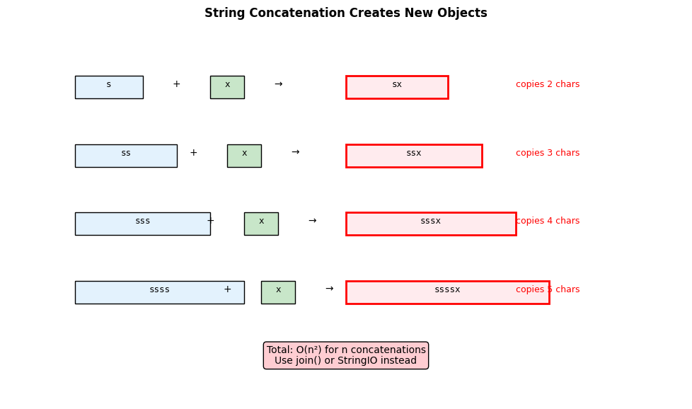
Building strings efficiently requires understanding concatenation costs.
import io
import timeit

n = 1000
chunk = "x" * 10

# Method 1: Repeated concatenation (BAD)
def build_concat():
    s = ""
    for _ in range(n):
        s += chunk  # Creates new string each time
    return s

# Method 2: Join (GOOD)
def build_join():
    parts = []
    for _ in range(n):
        parts.append(chunk)
    return "".join(parts)

# Method 3: StringIO (GOOD)
def build_io():
    buffer = io.StringIO()
    for _ in range(n):
        buffer.write(chunk)
    return buffer.getvalue()

# Compare performance
t1 = timeit.timeit(build_concat, number=100)
t2 = timeit.timeit(build_join, number=100)
t3 = timeit.timeit(build_io, number=100)

print(f"Building {n}-chunk string (100 iterations):")
print(f"  Concatenation: {t1:.4f}s")
print(f"  Join:          {t2:.4f}s ({t1/t2:.1f}x faster)")
print(f"  StringIO:      {t3:.4f}s ({t1/t3:.1f}x faster)")
Building 1000-chunk string (100 iterations):
  Concatenation: 0.0029s
  Join:          0.0015s (2.0x faster)
  StringIO:      0.0016s (1.8x faster)
Collection Internals: Sets and Frozen Sets
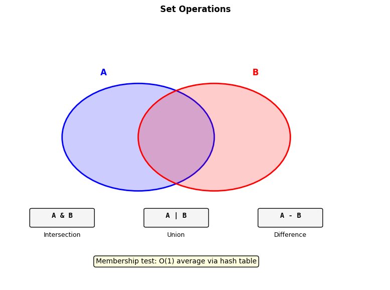
Sets use the same hash table technology as dictionaries, optimized for membership testing.
# Set performance demonstration
import random

# Create test data
numbers = list(range(10000))
random.shuffle(numbers)

test_list = numbers[:5000]
test_set = set(test_list)

# Membership testing
lookups = random.sample(range(10000), 100)

import time

# List lookup
start = time.perf_counter()
for x in lookups:
    _ = x in test_list
list_time = time.perf_counter() - start

# Set lookup
start = time.perf_counter()
for x in lookups:
    _ = x in test_set
set_time = time.perf_counter() - start

print(f"100 lookups in collection of 5000:")
print(f"  List: {list_time*1000:.3f} ms")
print(f"  Set:  {set_time*1000:.3f} ms")
print(f"  Speedup: {list_time/set_time:.1f}x")

# Set operations
a = {1, 2, 3, 4, 5}
b = {4, 5, 6, 7, 8}

print(f"\nSet operations:")
print(f"  a & b = {a & b}")  # Intersection
print(f"  a | b = {a | b}")  # Union
print(f"  a - b = {a - b}")  # Difference
print(f"  a ^ b = {a ^ b}")  # Symmetric difference
100 lookups in collection of 5000:
  List: 1.177 ms
  Set:  0.019 ms
  Speedup: 62.5x

Set operations:
  a & b = {4, 5}
  a | b = {1, 2, 3, 4, 5, 6, 7, 8}
  a - b = {1, 2, 3}
  a ^ b = {1, 2, 3, 6, 7, 8}
Set Implementation:
- Same hash table as dict (no values)
- Average O(1) for add, remove, membership
- Set operations optimized with early termination
- Frozen sets are immutable and hashable
When to use sets:
- Membership testing in loops
- Removing duplicates
- Mathematical set operations
- When order doesn’t matter
Memory overhead:
- Minimum size: 8 slots
- Growth factor: 4x until 50k, then 2x
- ~30% more memory than list of same items
Shallow vs Deep Copying
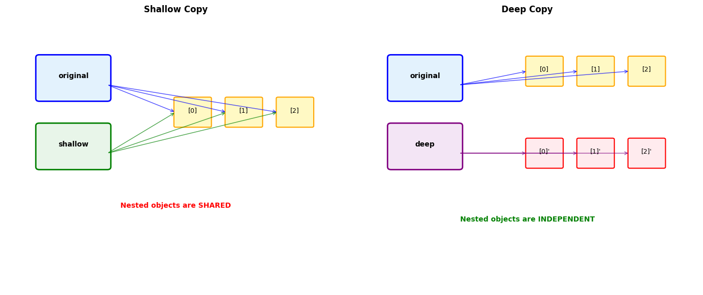
Python’s default copying behavior can lead to unexpected aliasing.
import copy

# Create nested structure
original = [[1, 2], [3, 4], [5, 6]]

# Different copy methods
reference = original
shallow = original.copy()  # or list(original) or original[:]
deep = copy.deepcopy(original)

# Modify nested object
original[0].append(3)

print("After modifying original[0]:")
print(f"  original:  {original}")
print(f"  reference: {reference}")  # Changed
print(f"  shallow:   {shallow}")    # Changed!
print(f"  deep:      {deep}")       # Unchanged

# Identity checks
print("\nIdentity comparisons:")
print(f"  original is reference: {original is reference}")
print(f"  original is shallow:   {original is shallow}")
print(f"  original[0] is shallow[0]: {original[0] is shallow[0]}")  # True!
print(f"  original[0] is deep[0]:    {original[0] is deep[0]}")     # False
After modifying original[0]:
  original:  [[1, 2, 3], [3, 4], [5, 6]]
  reference: [[1, 2, 3], [3, 4], [5, 6]]
  shallow:   [[1, 2, 3], [3, 4], [5, 6]]
  deep:      [[1, 2], [3, 4], [5, 6]]

Identity comparisons:
  original is reference: True
  original is shallow:   False
  original[0] is shallow[0]: True
  original[0] is deep[0]:    False
Composition vs Inheritance
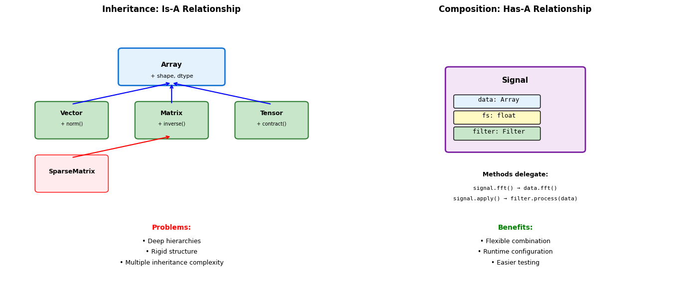
# Inheritance approach
class Vector(list):
    """Vector inherits from list."""

    def __init__(self, components):
        super().__init__(components)

    def magnitude(self):
        return sum(x**2 for x in self) ** 0.5

    def dot(self, other):
        return sum(a*b for a, b in zip(self, other))

# Problems with inheritance
v = Vector([3, 4])
print(f"Vector: {v}")
print(f"Magnitude: {v.magnitude()}")

# But inherits unwanted methods
v.reverse()  # Modifies in place!
print(f"After reverse: {v}")
v.append(5)  # Now 3D?
print(f"After append: {v}")
Vector: [3, 4]
Magnitude: 5.0
After reverse: [4, 3]
After append: [4, 3, 5]
# Composition approach
class Signal:
    """Signal uses composition."""

    def __init__(self, data, sample_rate):
        self._data = np.array(data)
        self.fs = sample_rate
        self._filter = None

    def __len__(self):
        return len(self._data)

    def __getitem__(self, idx):
        return self._data[idx]

    @property
    def duration(self):
        return len(self._data) / self.fs

    def fft(self):
        """Delegate to NumPy."""
        return np.fft.fft(self._data)

    def resample(self, new_rate):
        """Return new Signal."""
        ratio = new_rate / self.fs
        new_length = int(len(self._data) * ratio)
        new_data = np.interp(
            np.linspace(0, len(self._data), new_length),
            np.arange(len(self._data)),
            self._data
        )
        return Signal(new_data, new_rate)

# Clean interface
sig = Signal([1, 2, 3, 4], sample_rate=100)
print(f"Duration: {sig.duration}s")
print(f"FFT shape: {sig.fft().shape}")
Duration: 0.04s
FFT shape: (4,)
Object Creation and Initialization
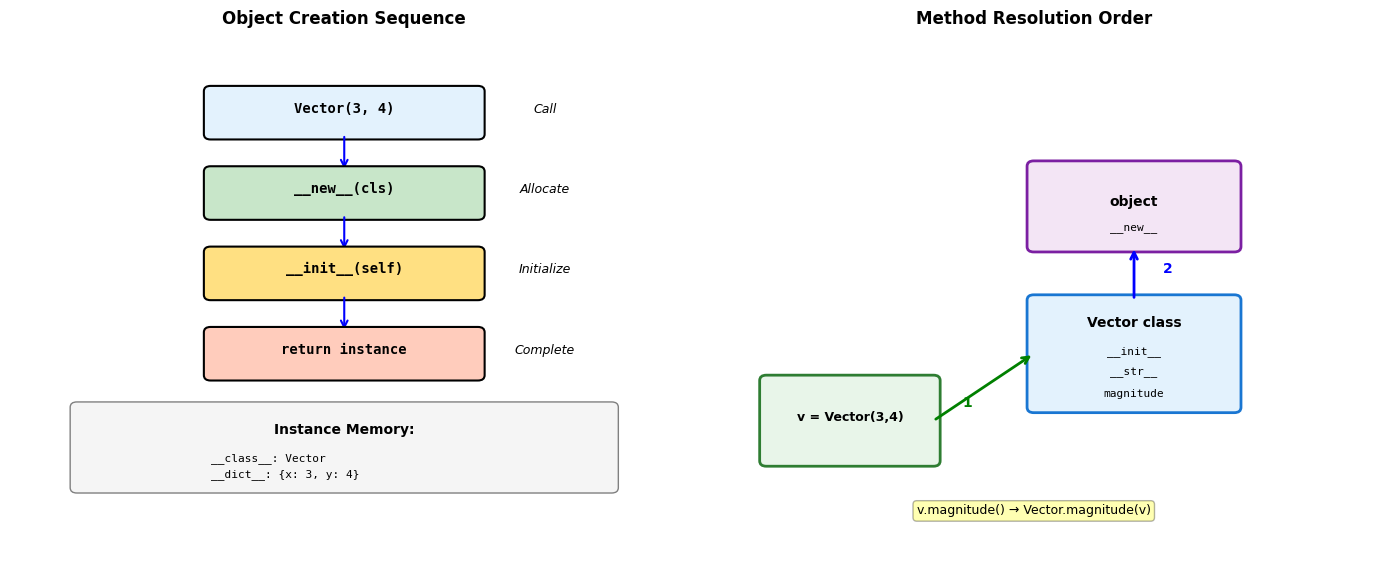
class Vector:
    """2D vector with special methods."""

    def __init__(self, x, y):
        """Initialize instance attributes."""
        self.x = x
        self.y = y

    def __repr__(self):
        """Developer representation (for debugging)."""
        return f"Vector({self.x}, {self.y})"

    def __str__(self):
        """User-friendly string representation."""
        return f"<{self.x}, {self.y}>"

    def magnitude(self):
        """Compute vector magnitude."""
        return (self.x**2 + self.y**2) ** 0.5

# Create instance
v = Vector(3, 4)

# Different string representations
print(f"repr(v): {repr(v)}")
print(f"str(v): {str(v)}")
print(f"Magnitude: {v.magnitude()}")

# Instance internals
print(f"\nInstance dict: {v.__dict__}")
print(f"Class: {v.__class__.__name__}")
repr(v): Vector(3, 4)
str(v): <3, 4>
Magnitude: 5.0

Instance dict: {'x': 3, 'y': 4}
Class: Vector
# Method resolution demonstration
class Base:
    def method(self):
        return "Base"

    def override_me(self):
        return "Base version"

class Derived(Base):
    def override_me(self):
        return "Derived version"

    def method(self):
        # Call parent version
        parent = super().method()
        return f"{parent} → Derived"

d = Derived()
print(f"d.override_me(): {d.override_me()}")
print(f"d.method(): {d.method()}")

# MRO (Method Resolution Order)
print(f"\nMRO: {[cls.__name__ for cls in Derived.__mro__]}")

# Bound vs unbound methods
print(f"\nBound method: {d.method}")
print(f"Unbound: {Derived.method}")
print(f"Same function: {d.method.__func__ is Derived.method}")
d.override_me(): Derived version
d.method(): Base → Derived

MRO: ['Derived', 'Base', 'object']

Bound method: <bound method Derived.method of <__main__.Derived object at 0x10b62a270>>
Unbound: <function Derived.method at 0x10cb16a20>
Same function: True
Operator Overloading for Numerical Types
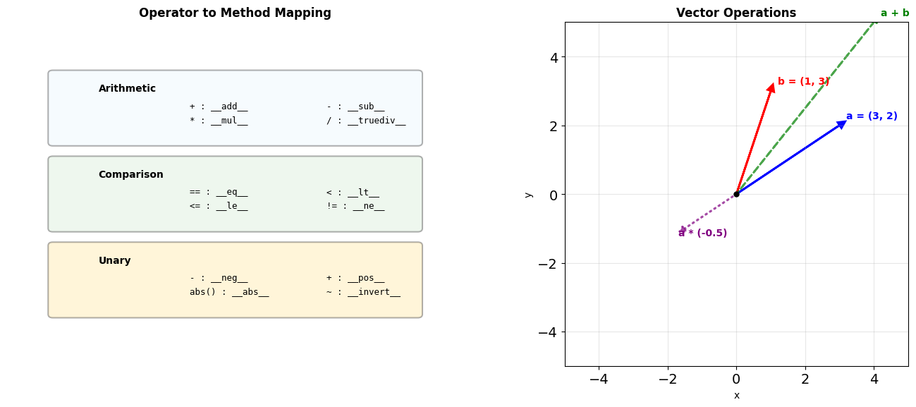
class Vector:
    def __init__(self, x, y):
        self.x = x
        self.y = y

    def __repr__(self):
        return f"Vector({self.x}, {self.y})"

    # Arithmetic operators
    def __add__(self, other):
        if isinstance(other, Vector):
            return Vector(self.x + other.x, self.y + other.y)
        return NotImplemented

    def __mul__(self, scalar):
        if isinstance(scalar, (int, float)):
            return Vector(self.x * scalar, self.y * scalar)
        return NotImplemented

    def __rmul__(self, scalar):
        """Right multiplication: scalar * vector"""
        return self.__mul__(scalar)

    def __neg__(self):
        return Vector(-self.x, -self.y)

    def __abs__(self):
        return (self.x**2 + self.y**2) ** 0.5

    # Comparison operators
    def __eq__(self, other):
        if not isinstance(other, Vector):
            return False
        return self.x == other.x and self.y == other.y

    def __lt__(self, other):
        """Compare by magnitude."""
        return abs(self) < abs(other)

# Usage
a = Vector(3, 4)
b = Vector(1, 2)

print(f"a = {a}")
print(f"b = {b}")
print(f"a + b = {a + b}")
print(f"2 * a = {2 * a}")
print(f"-a = {-a}")
print(f"|a| = {abs(a)}")
print(f"a == b: {a == b}")
print(f"a > b: {a > b}")
a = Vector(3, 4)
b = Vector(1, 2)
a + b = Vector(4, 6)
2 * a = Vector(6, 8)
-a = Vector(-3, -4)
|a| = 5.0
a == b: False
a > b: True
# In-place operators
class Matrix:
    def __init__(self, data):
        self.data = np.array(data, dtype=float)

    def __repr__(self):
        return f"Matrix({self.data.tolist()})"

    def __iadd__(self, other):
        """In-place addition: m += other"""
        if isinstance(other, Matrix):
            self.data += other.data
        elif isinstance(other, (int, float)):
            self.data += other
        else:
            return NotImplemented
        return self  # Must return self

    def __matmul__(self, other):
        """Matrix multiplication: m @ other"""
        if isinstance(other, Matrix):
            return Matrix(self.data @ other.data)
        return NotImplemented

    def __getitem__(self, key):
        """Indexing: m[i, j]"""
        return self.data[key]

    def __setitem__(self, key, value):
        """Assignment: m[i, j] = value"""
        self.data[key] = value

# Usage
m1 = Matrix([[1, 2], [3, 4]])
m2 = Matrix([[5, 6], [7, 8]])

print(f"m1 = {m1}")
print(f"m2 = {m2}")
print(f"m1 @ m2 = {m1 @ m2}")
print(f"m1[0, 1] = {m1[0, 1]}")

m1 += 10
print(f"After m1 += 10: {m1}")
m1 = Matrix([[1.0, 2.0], [3.0, 4.0]])
m2 = Matrix([[5.0, 6.0], [7.0, 8.0]])
m1 @ m2 = Matrix([[19.0, 22.0], [43.0, 50.0]])
m1[0, 1] = 2.0
After m1 += 10: Matrix([[11.0, 12.0], [13.0, 14.0]])
Properties and Descriptors
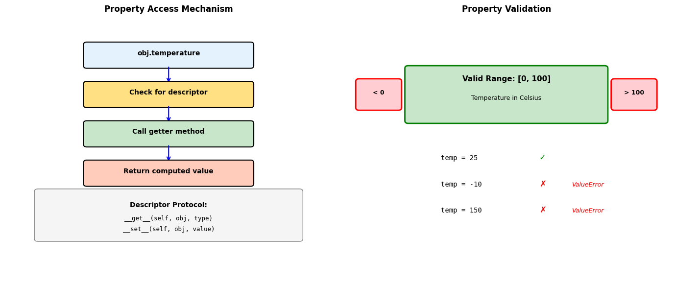
class Temperature:
    """Temperature with Celsius/Fahrenheit properties."""

    def __init__(self, celsius=0):
        self._celsius = celsius

    @property
    def celsius(self):
        """Getter for Celsius."""
        return self._celsius

    @celsius.setter
    def celsius(self, value):
        """Setter with validation."""
        if value < -273.15:
            raise ValueError(f"Temperature below absolute zero")
        self._celsius = value

    @property
    def fahrenheit(self):
        """Computed Fahrenheit property."""
        return self._celsius * 9/5 + 32

    @fahrenheit.setter
    def fahrenheit(self, value):
        """Set via Fahrenheit."""
        self.celsius = (value - 32) * 5/9

    @property
    def kelvin(self):
        """Read-only Kelvin property."""
        return self._celsius + 273.15

# Usage
temp = Temperature(25)
print(f"Celsius: {temp.celsius}°C")
print(f"Fahrenheit: {temp.fahrenheit}°F")
print(f"Kelvin: {temp.kelvin}K")

temp.fahrenheit = 86
print(f"\nAfter setting 86°F:")
print(f"Celsius: {temp.celsius}°C")

try:
    temp.celsius = -300
except ValueError as e:
    print(f"\nValidation error: {e}")
Celsius: 25°C
Fahrenheit: 77.0°F
Kelvin: 298.15K

After setting 86°F:
Celsius: 30.0°C

Validation error: Temperature below absolute zero
When to use properties:
- Computed values derived from other attributes
- Validation on attribute assignment
- Converting between representations (e.g., Celsius/Fahrenheit)
- Read-only attributes that shouldn’t be modified
Property mechanics:
- Getter: Called on
obj.attraccess - Setter: Called on
obj.attr = valueassignment - Deleter: Called on
del obj.attr - Properties are descriptors under the hood
Class vs Instance Attributes
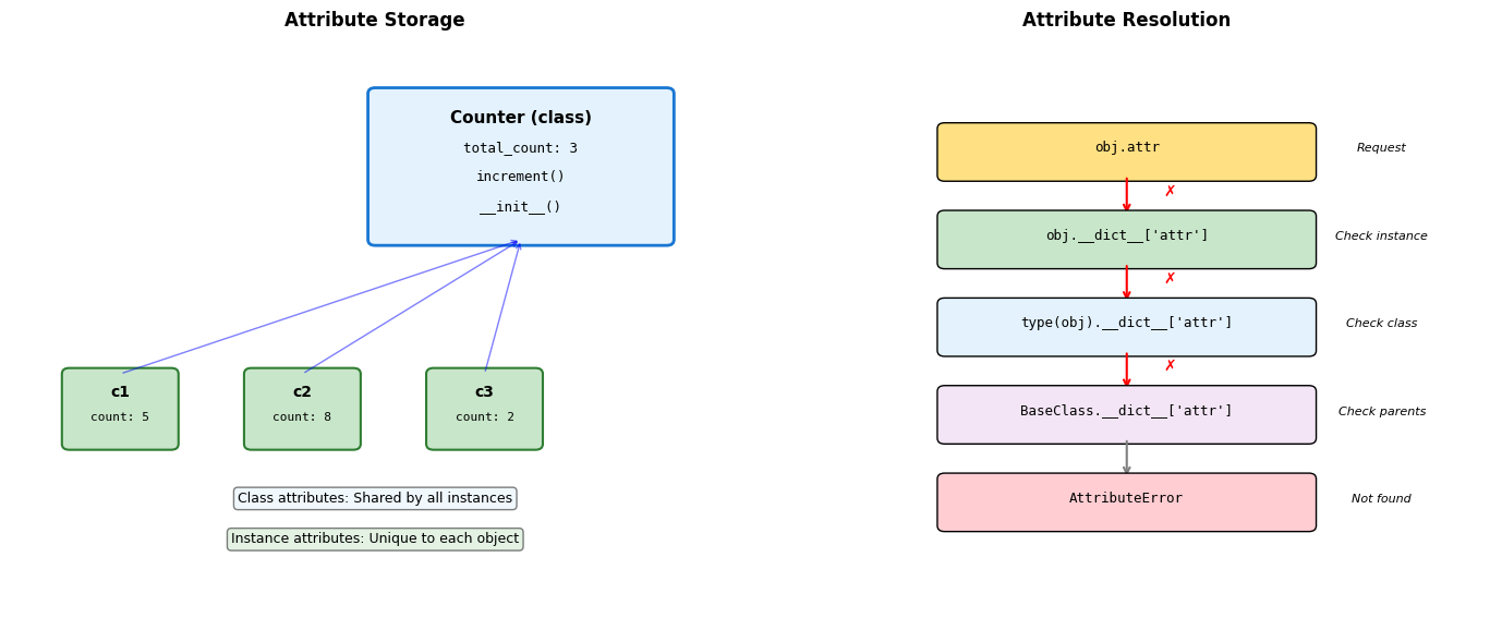
class Counter:
    """Demonstrates class vs instance attributes."""

    # Class attribute (shared)
    total_instances = 0
    default_step = 1

    def __init__(self, initial=0):
        # Instance attributes (unique)
        self.count = initial
        Counter.total_instances += 1

    def increment(self, step=None):
        # Use class default if not specified
        if step is None:
            step = self.default_step
        self.count += step

    @classmethod
    def get_total(cls):
        """Class method accesses class attributes."""
        return cls.total_instances

    @staticmethod
    def validate_step(step):
        """Static method - no access to instance or class."""
        return step > 0

# Create instances
c1 = Counter()
c2 = Counter(10)
c3 = Counter(20)

print(f"Total instances: {Counter.total_instances}")
print(f"c1.count: {c1.count}")
print(f"c2.count: {c2.count}")

# Modify class attribute
Counter.default_step = 5
c1.increment()
c2.increment()

print(f"\nAfter increment with step=5:")
print(f"c1.count: {c1.count}")
print(f"c2.count: {c2.count}")

# Instance shadows class attribute
c1.default_step = 10
print(f"\nc1.default_step: {c1.default_step}")
print(f"c2.default_step: {c2.default_step}")
Total instances: 3
c1.count: 0
c2.count: 10

After increment with step=5:
c1.count: 5
c2.count: 15

c1.default_step: 10
c2.default_step: 5
Class vs instance attributes:
- Class attributes: Shared by all instances, defined at class level
- Instance attributes: Unique to each object, defined in
__init__ - Instance attributes shadow class attributes of the same name
Method types:
- Instance methods:
selfas first argument, access instance state - Class methods (
@classmethod):clsas first argument, access class state - Static methods (
@staticmethod): No implicit argument, utility functions
Common patterns:
- Class-level defaults modified per-instance
- Instance counters via class attributes
- Factory methods via
@classmethod
Abstract Base Classes and Protocols
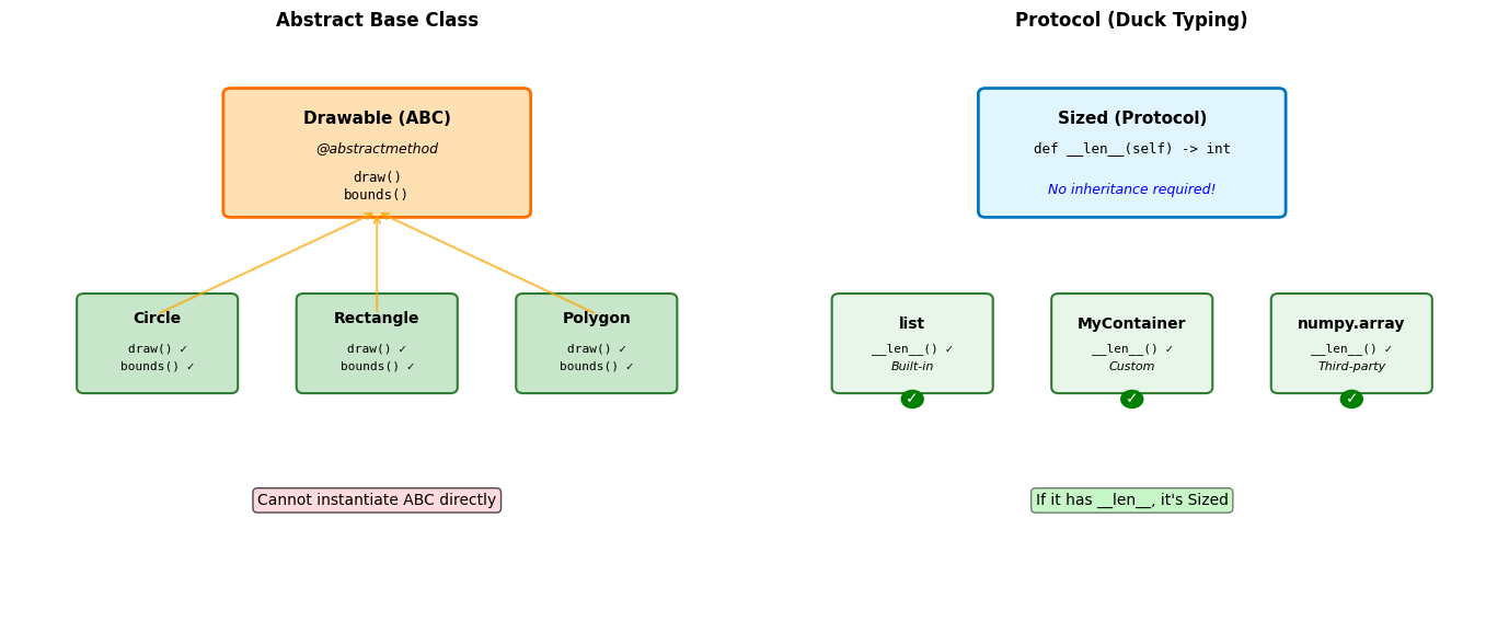
from abc import ABC, abstractmethod
import math

class Shape(ABC):
    """Abstract base class for shapes."""

    @abstractmethod
    def area(self):
        """Must be implemented by subclasses."""
        pass

    @abstractmethod
    def perimeter(self):
        """Must be implemented by subclasses."""
        pass

    def describe(self):
        """Concrete method using abstract methods."""
        return f"Area: {self.area():.2f}, Perimeter: {self.perimeter():.2f}"

class Circle(Shape):
    def __init__(self, radius):
        self.radius = radius

    def area(self):
        return math.pi * self.radius ** 2

    def perimeter(self):
        return 2 * math.pi * self.radius

class Rectangle(Shape):
    def __init__(self, width, height):
        self.width = width
        self.height = height

    def area(self):
        return self.width * self.height

    def perimeter(self):
        return 2 * (self.width + self.height)

# Cannot instantiate ABC
try:
    shape = Shape()  # Error!
except TypeError as e:
    print(f"Error: {e}")

# Concrete classes work
circle = Circle(5)
rect = Rectangle(3, 4)

print(f"\nCircle: {circle.describe()}")
print(f"Rectangle: {rect.describe()}")

# Check inheritance
print(f"\nisinstance(circle, Shape): {isinstance(circle, Shape)}")
Error: Can't instantiate abstract class Shape without an implementation for abstract methods 'area', 'perimeter'

Circle: Area: 78.54, Perimeter: 31.42
Rectangle: Area: 12.00, Perimeter: 14.00

isinstance(circle, Shape): True
When to use ABCs:
- Defining interfaces that must be implemented
- Template Method pattern (concrete methods calling abstract ones)
- Enforcing contracts in a class hierarchy
- When you want
isinstance()checks against the interface
ABC vs Duck Typing:
- ABCs: Explicit contracts, errors at instantiation time
- Duck typing: Implicit contracts, errors at call time
- Python prefers duck typing, but ABCs useful for frameworks
Built-in ABCs (collections.abc):
Iterable,Iterator,SequenceMapping,MutableMappingCallable,Hashable
Dataclasses for Numerical Structures
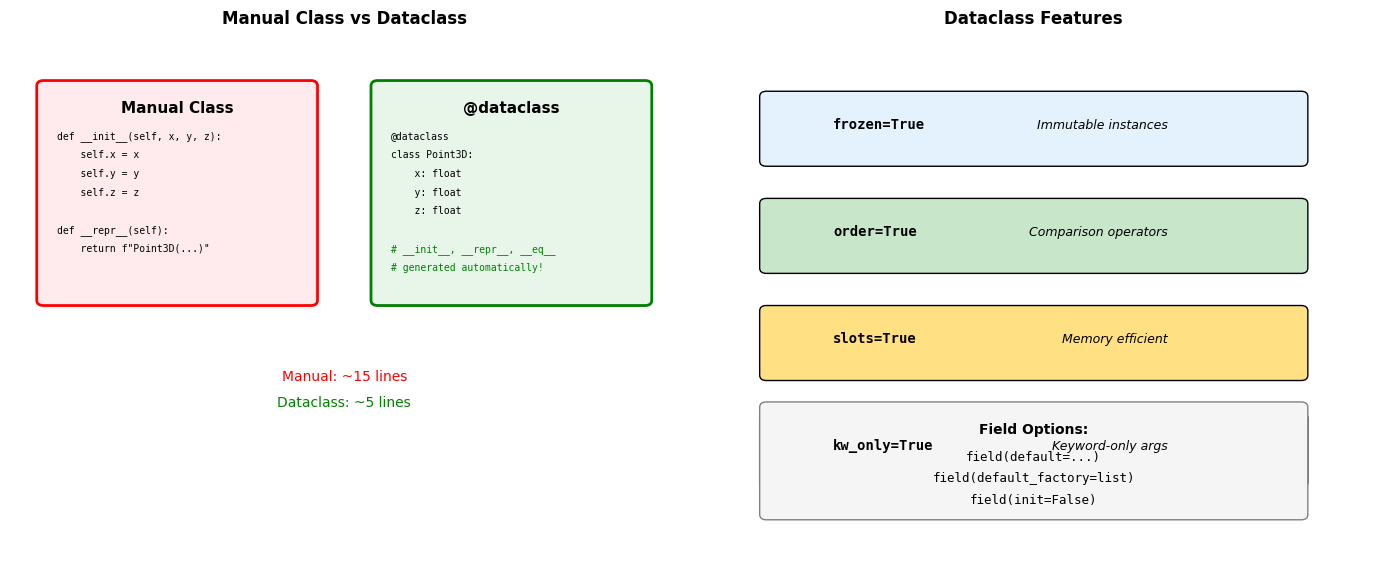
from dataclasses import dataclass, field
from typing import List
import numpy as np

@dataclass
class DataPoint:
    """Simple data container."""
    x: float
    y: float
    label: str = "unlabeled"
    metadata: dict = field(default_factory=dict)

    def distance_to(self, other):
        """Euclidean distance."""
        return ((self.x - other.x)**2 +
                (self.y - other.y)**2) ** 0.5

@dataclass(frozen=True)
class ImmutableVector:
    """Frozen dataclass - hashable."""
    x: float
    y: float
    z: float

    def magnitude(self):
        return (self.x**2 + self.y**2 + self.z**2) ** 0.5

    def __add__(self, other):
        """Return new vector (immutable)."""
        return ImmutableVector(
            self.x + other.x,
            self.y + other.y,
            self.z + other.z
        )

# Usage
p1 = DataPoint(3, 4)
p2 = DataPoint(6, 8, "target")

print(f"p1: {p1}")
print(f"p2: {p2}")
print(f"Distance: {p1.distance_to(p2):.2f}")

# Frozen vector
v1 = ImmutableVector(1, 2, 3)
v2 = ImmutableVector(4, 5, 6)
v3 = v1 + v2

print(f"\nv1 + v2 = {v3}")
print(f"Hashable: {hash(v1)}")

# Can use as dict key
vector_dict = {v1: "first", v2: "second"}
p1: DataPoint(x=3, y=4, label='unlabeled', metadata={})
p2: DataPoint(x=6, y=8, label='target', metadata={})
Distance: 5.00

v1 + v2 = ImmutableVector(x=5, y=7, z=9)
Hashable: 529344067295497451
@dataclass(order=True)
class Measurement:
    """Sortable measurement with validation."""
    timestamp: float = field(compare=True)
    value: float = field(compare=False)
    sensor_id: str = field(default="unknown", compare=False)

    def __post_init__(self):
        """Validation after initialization."""
        if self.value < 0:
            raise ValueError(f"Negative value: {self.value}")
        if self.timestamp < 0:
            raise ValueError(f"Invalid timestamp: {self.timestamp}")

# Sorting by timestamp
measurements = [
    Measurement(100.5, 23.4, "A1"),
    Measurement(99.2, 25.1, "A2"),
    Measurement(101.3, 22.8, "A1"),
]

sorted_measurements = sorted(measurements)
print("Sorted by timestamp:")
for m in sorted_measurements:
    print(f"  t={m.timestamp}: {m.value}")

# Performance comparison
from dataclasses import dataclass
import sys

@dataclass(slots=True)
class SlottedPoint:
    x: float
    y: float

@dataclass
class RegularPoint:
    x: float
    y: float

sp = SlottedPoint(1, 2)
rp = RegularPoint(1, 2)

print(f"\nMemory usage:")
print(f"  With slots: {sys.getsizeof(sp)} bytes")
print(f"  Regular: {sys.getsizeof(rp) + sys.getsizeof(rp.__dict__)} bytes")
Sorted by timestamp:
  t=99.2: 25.1
  t=100.5: 23.4
  t=101.3: 22.8

Memory usage:
  With slots: 48 bytes
  Regular: 344 bytes
The Python Scientific Stack
Python’s numerical libraries form a layered stack. Each layer builds on the ones below, trading some performance for convenience and expressiveness.
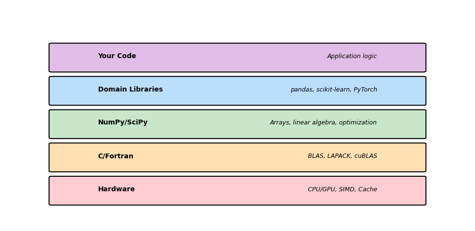
Each layer provides:
- Higher-level abstractions
- Automatic optimizations
- Platform independence
- Tested, maintained code
The goal: Write code at the highest appropriate level. Let NumPy/SciPy call optimized C/Fortran for you.
Example: Matrix multiply
# Don't write this
result = [[0]*n for _ in range(n)]
for i in range(n):
    for j in range(n):
        for k in range(n):
            result[i][j] += A[i][k] * B[k][j]

# Write this
result = A @ B  # Calls optimized BLAS
NumPy’s @ operator uses BLAS libraries that exploit CPU features (SIMD, cache blocking, parallelism).
Why NumPy Exists: Python’s Performance Wall
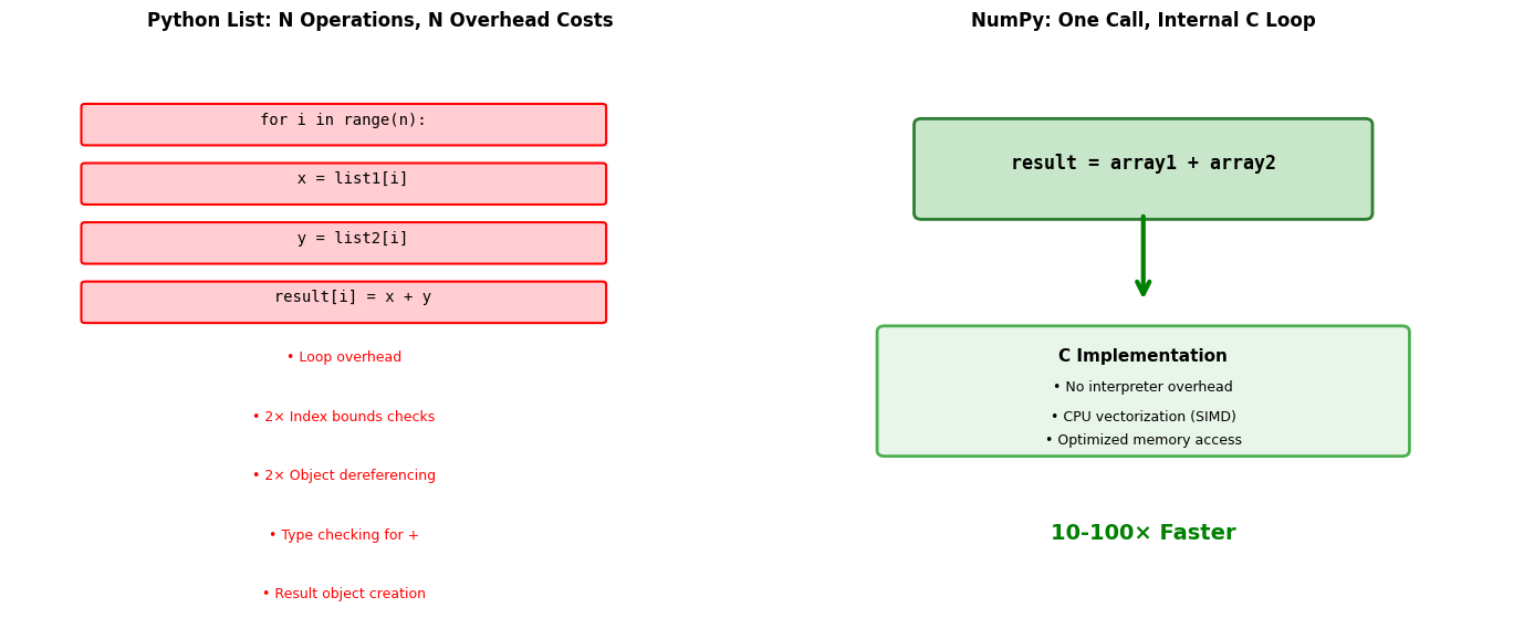
NumPy solves Python’s fundamental limitation: every operation triggers expensive interpreter overhead.
import numpy as np
import timeit

# Demonstrate the performance difference
def python_add(list1, list2):
    """Pure Python element-wise addition."""
    result = []
    for i in range(len(list1)):
        result.append(list1[i] + list2[i])
    return result

def numpy_add(arr1, arr2):
    """NumPy vectorized addition."""
    return arr1 + arr2

# Test data
size = 100000
py_list1 = list(range(size))
py_list2 = list(range(size, size*2))
np_arr1 = np.array(py_list1)
np_arr2 = np.array(py_list2)

# Benchmark
t_python = timeit.timeit(
    lambda: python_add(py_list1, py_list2),
    number=10
)
t_numpy = timeit.timeit(
    lambda: numpy_add(np_arr1, np_arr2),
    number=10
)

print(f"Adding {size:,} numbers (10 iterations):")
print(f"  Python lists: {t_python:.3f}s")
print(f"  NumPy arrays: {t_numpy:.3f}s")
print(f"  Speedup: {t_python/t_numpy:.0f}x")

# Show function call overhead
python_ops = size * 4  # loop, 2 indexes, 1 addition per iteration
numpy_ops = 1  # single function call
print(f"\nPython operations: {python_ops:,}")
print(f"NumPy operations: {numpy_ops}")
print(f"Overhead reduction: {python_ops/numpy_ops:.0f}x")
Adding 100,000 numbers (10 iterations):
  Python lists: 0.022s
  NumPy arrays: 0.000s
  Speedup: 69x

Python operations: 400,000
NumPy operations: 1
Overhead reduction: 400000x
The NumPy Solution:
- Homogeneous data - All elements same type, enabling compact storage
- Contiguous memory - Cache-friendly access patterns
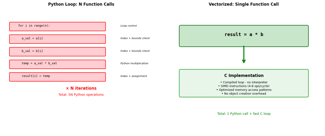
- Vectorized operations - Single Python call processes entire arrays
- C implementation - Inner loops run at machine speed
Cost of flexibility:
- Python lists can mix types, NumPy arrays cannot
- Dynamic resizing is expensive in NumPy
- Small arrays may be slower due to overhead
When NumPy wins:
- Numerical computations on large datasets
- Element-wise operations
- Mathematical functions (sin, cos, exp)
- Linear algebra operations
Array Object Internals: More Than Just Data
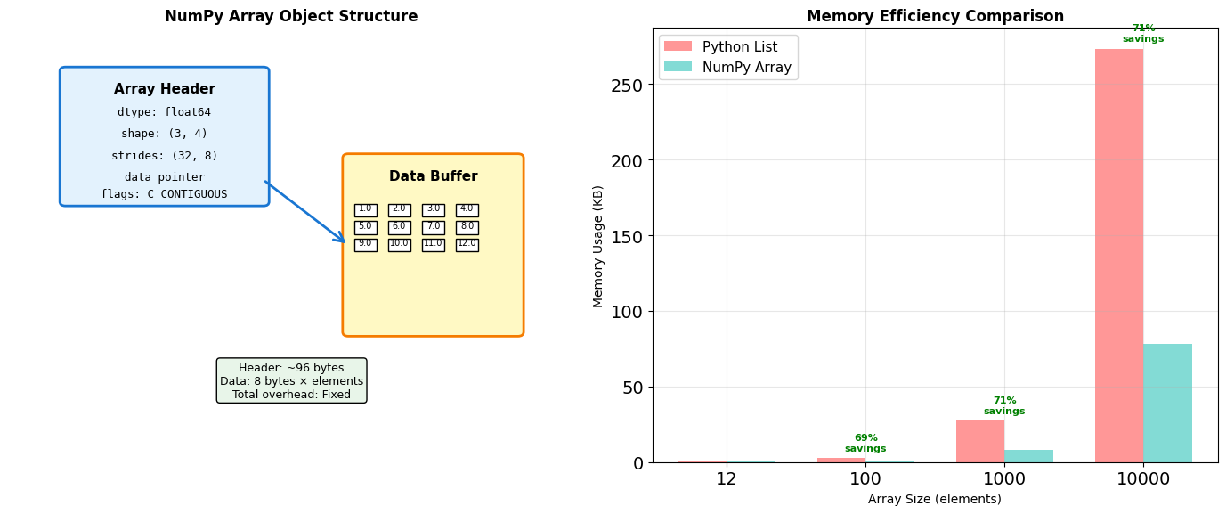
NumPy arrays separate metadata from data, enabling views and broadcasting without copying.
import numpy as np
import sys

# Examine array internals
arr = np.arange(12, dtype=np.float64).reshape(3, 4)

print("Array structure analysis:")
print(f"  Array object size: {sys.getsizeof(arr)} bytes")
print(f"  Data buffer size: {arr.nbytes} bytes")
print(f"  Shape: {arr.shape}")
print(f"  Strides: {arr.strides}")  # Bytes to next element in each dimension
print(f"  Data type: {arr.dtype}")
print(f"  Item size: {arr.itemsize} bytes")

# Memory layout inspection
print(f"\nMemory layout:")
print(f"  C-contiguous: {arr.flags['C_CONTIGUOUS']}")
print(f"  F-contiguous: {arr.flags['F_CONTIGUOUS']}")
print(f"  Owns data: {arr.flags['OWNDATA']}")

# Compare with Python list
py_list = arr.tolist()
print(f"\nMemory comparison for 12 elements:")
print(f"  NumPy array: {sys.getsizeof(arr) + arr.nbytes} bytes total")
print(f"  Python list: {sys.getsizeof(py_list)} bytes (list)")

# Calculate Python list element overhead
element_overhead = sum(sys.getsizeof(x) for row in py_list for x in row)
print(f"  Python objects: {element_overhead} bytes (elements)")
print(f"  Python total: {sys.getsizeof(py_list) + element_overhead} bytes")

# Show memory addressing
print(f"\nMemory addressing:")
print(f"  Base address: {arr.__array_interface__['data'][0]:#x}")
print(f"  Element [0,0] offset: 0 bytes")
print(f"  Element [0,1] offset: {arr.strides[1]} bytes")
print(f"  Element [1,0] offset: {arr.strides[0]} bytes")

# Demonstrate stride calculation
row, col = 1, 2
offset = row * arr.strides[0] + col * arr.strides[1]
print(f"  Element [1,2] offset: {offset} bytes → value {arr[1,2]}")
Array structure analysis:
  Array object size: 128 bytes
  Data buffer size: 96 bytes
  Shape: (3, 4)
  Strides: (32, 8)
  Data type: float64
  Item size: 8 bytes

Memory layout:
  C-contiguous: True
  F-contiguous: False
  Owns data: False

Memory comparison for 12 elements:
  NumPy array: 224 bytes total
  Python list: 80 bytes (list)
  Python objects: 288 bytes (elements)
  Python total: 368 bytes

Memory addressing:
  Base address: 0x6000000dd440
  Element [0,0] offset: 0 bytes
  Element [0,1] offset: 8 bytes
  Element [1,0] offset: 32 bytes
  Element [1,2] offset: 48 bytes → value 6.0
Array metadata enables:
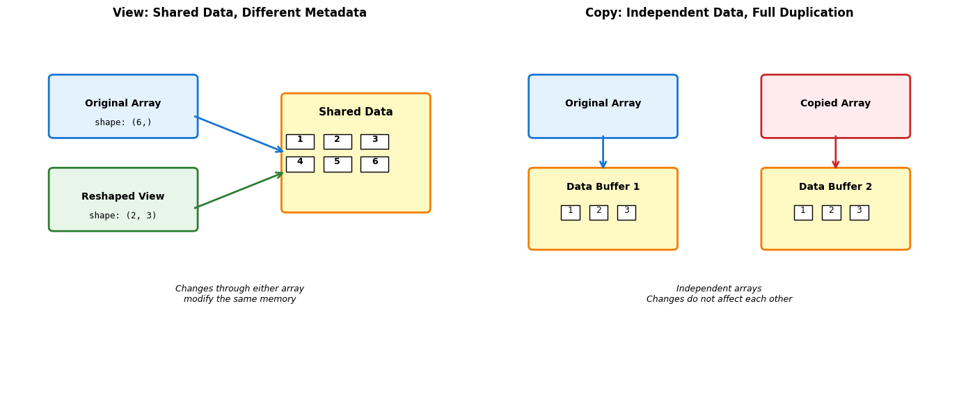
- Reshaping without copying - Same data, different view
- Slicing creates views - No memory duplication
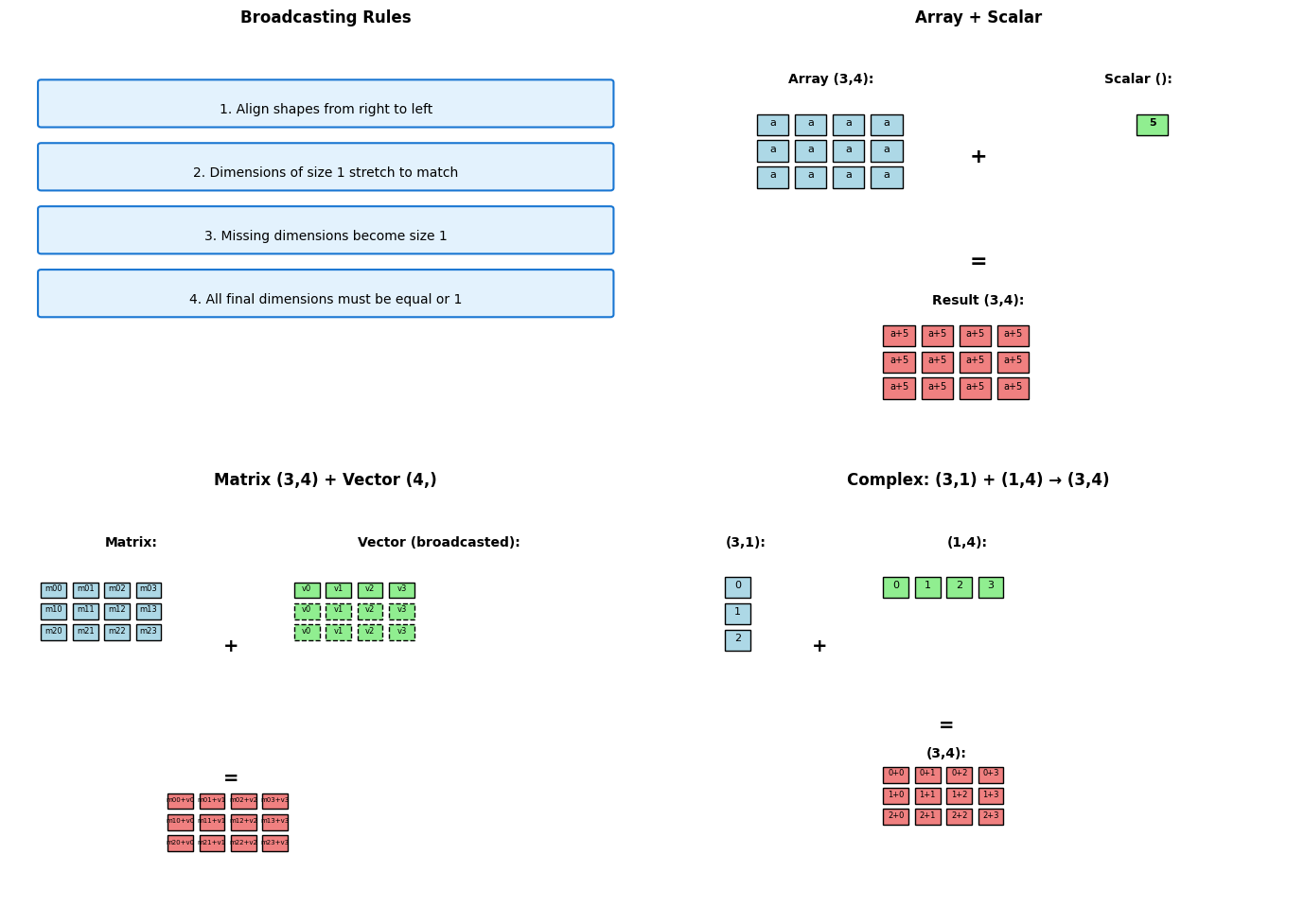
- Broadcasting - Operations on different-shaped arrays
- Memory mapping - Work with files larger than RAM
Memory Layout: Row-Major vs Column-Major
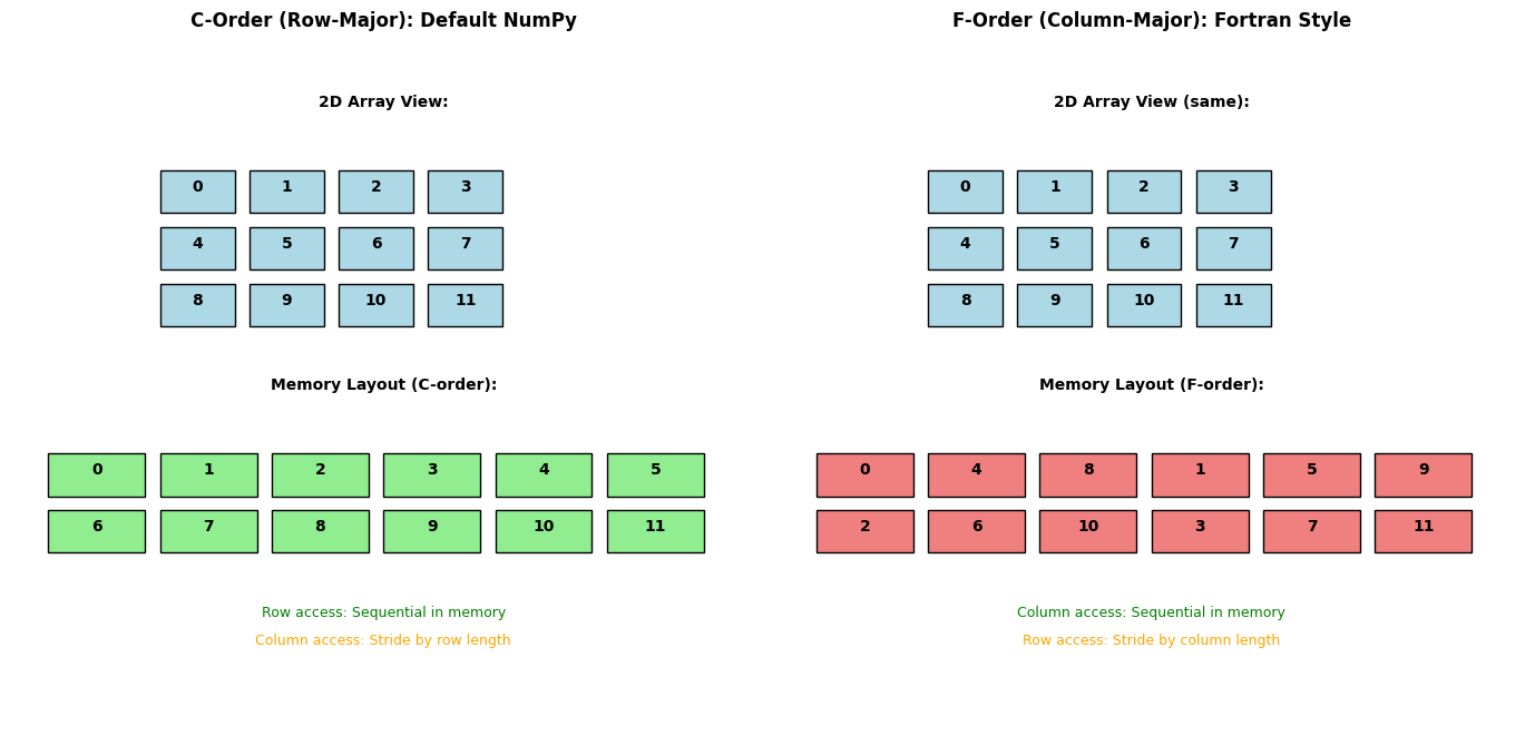
Array element ordering in memory affects performance significantly due to CPU cache behavior.
import numpy as np
import timeit

# Create arrays with different memory layouts
size = 1000
c_array = np.random.rand(size, size)  # C-order (default)
f_array = np.asfortranarray(c_array)  # F-order copy

print("Memory layout comparison:")
print(f"C-order shape: {c_array.shape}, strides: {c_array.strides}")
print(f"F-order shape: {f_array.shape}, strides: {f_array.strides}")
print(f"C-order flags: C={c_array.flags.c_contiguous}, F={c_array.flags.f_contiguous}")
print(f"F-order flags: C={f_array.flags.c_contiguous}, F={f_array.flags.f_contiguous}")

# Row access performance (C-order wins)
def sum_rows(arr):
    return [np.sum(arr[i, :]) for i in range(100)]

# Column access performance (F-order wins)
def sum_cols(arr):
    return [np.sum(arr[:, j]) for j in range(100)]

t_c_rows = timeit.timeit(lambda: sum_rows(c_array), number=100)
t_f_rows = timeit.timeit(lambda: sum_rows(f_array), number=100)

t_c_cols = timeit.timeit(lambda: sum_cols(c_array), number=100)
t_f_cols = timeit.timeit(lambda: sum_cols(f_array), number=100)

print(f"\nRow access performance (100 iterations):")
print(f"  C-order: {t_c_rows:.3f}s")
print(f"  F-order: {t_f_rows:.3f}s ({t_f_rows/t_c_rows:.1f}x slower)")

print(f"\nColumn access performance (100 iterations):")
print(f"  C-order: {t_c_cols:.3f}s")
print(f"  F-order: {t_f_cols:.3f}s ({t_c_cols/t_f_cols:.1f}x faster)")
Memory layout comparison:
C-order shape: (1000, 1000), strides: (8000, 8)
F-order shape: (1000, 1000), strides: (8, 8000)
C-order flags: C=True, F=False
F-order flags: C=False, F=True

Row access performance (100 iterations):
  C-order: 0.010s
  F-order: 0.013s (1.3x slower)

Column access performance (100 iterations):
  C-order: 0.012s
  F-order: 0.010s (1.2x faster)
Memory layout matters because:
- CPU cache lines - Fetch 64-byte chunks from RAM
- Spatial locality - Adjacent memory access is faster
- Prefetching - CPU predicts sequential access patterns
C-order (row-major):
- Default in NumPy, C, Python
- Rows stored contiguously
- Better for row operations
F-order (column-major):
- Default in Fortran, MATLAB, R
- Columns stored contiguously
- Better for column operations
- Required by some BLAS routines
Performance implications:
- Cache misses can cause 100× slowdowns
- Matrix algorithms should match layout
- Transpose operations may change layout
Views vs Copies: Memory Management Semantics
NumPy operations can either create views (sharing data) or copies (duplicating data).
import numpy as np

# Create original array
original = np.arange(12).reshape(3, 4)
print("Original array:")
print(original)

# View operations (share data)
view_reshaped = original.reshape(4, 3)
view_slice = original[1:, :]
view_transpose = original.T

print(f"\nView operations (share data):")
print(f"  original.base is None: {original.base is None}")
print(f"  view_reshaped.base is original: {view_reshaped.base is original}")
print(f"  view_slice.base is original: {view_slice.base is original}")
print(f"  view_transpose.base is original: {view_transpose.base is original}")

# Test sharing - modify through view
original[0, 0] = 999
print(f"\nAfter setting original[0,0] = 999:")
print(f"  original[0,0] = {original[0,0]}")
print(f"  view_reshaped[0,0] = {view_reshaped[0,0]}")  # Same memory!

# Copy operations (independent data)
copy_array = original.copy()
copy_flatten = original.flatten()  # Unlike ravel(), always copies

print(f"\nCopy operations (independent data):")
print(f"  copy_array.base is None: {copy_array.base is None}")
print(f"  copy_flatten.base is None: {copy_flatten.base is None}")

# Test independence
original[1, 1] = 888
print(f"\nAfter setting original[1,1] = 888:")
print(f"  original[1,1] = {original[1,1]}")
print(f"  copy_array[1,1] = {copy_array[1,1]}")  # Independent!

# Memory usage comparison
import sys
print(f"\nMemory usage:")
print(f"  Original: {original.nbytes} bytes")
print(f"  View: {view_reshaped.nbytes} bytes data (shares with original)")
print(f"  Copy: {copy_array.nbytes} bytes (independent)")
print(f"  Total with view: ~{original.nbytes} bytes")
print(f"  Total with copy: ~{original.nbytes + copy_array.nbytes} bytes")

# Dangerous view scenario
def demonstrate_view_trap():
    """Common mistake with views."""
    data = np.arange(10)
    subset = data[::2]  # Every other element (view)

    # Modify original
    data.fill(0)

    return subset  # Returns modified data!

result = demonstrate_view_trap()
print(f"\nView trap result: {result}")  # All zeros, not original values!
Original array:
[[ 0  1  2  3]
 [ 4  5  6  7]
 [ 8  9 10 11]]

View operations (share data):
  original.base is None: False
  view_reshaped.base is original: False
  view_slice.base is original: False
  view_transpose.base is original: False

After setting original[0,0] = 999:
  original[0,0] = 999
  view_reshaped[0,0] = 999

Copy operations (independent data):
  copy_array.base is None: True
  copy_flatten.base is None: True

After setting original[1,1] = 888:
  original[1,1] = 888
  copy_array[1,1] = 5

Memory usage:
  Original: 96 bytes
  View: 96 bytes data (shares with original)
  Copy: 96 bytes (independent)
  Total with view: ~96 bytes
  Total with copy: ~192 bytes

View trap result: [0 0 0 0 0]
View operations (share data):
- Slicing:
arr[start:stop] - Reshaping:
arr.reshape() - Transposing:
arr.T - Index arrays with step:
arr[::2]
Copy operations (new data):
- Explicit copy:
arr.copy() - Fancy indexing:
arr[[1,3,5]] - Boolean indexing:
arr[arr > 0] - Some functions:
flatten(),ravel()(conditionally)
Broadcasting: Operations on Different-Shaped Arrays
Broadcasting enables operations between arrays of different shapes without explicit loops or memory duplication.
import numpy as np

# Broadcasting examples with shape analysis
def show_broadcast(a, b, operation_name):
    """Demonstrate broadcasting between two arrays."""
    print(f"\n{operation_name}:")
    print(f"  Array A shape: {a.shape}")

    # Handle scalar case
    if np.isscalar(b):
        print(f"  Array B: scalar ({b})")
        b_bytes = 8  # Approximate scalar size
    else:
        print(f"  Array B shape: {b.shape}")
        b_bytes = b.nbytes

    try:
        result = a + b
        print(f"  Result shape: {result.shape}")
        print(f"  Memory usage: A={a.nbytes}B, B={b_bytes}B, Result={result.nbytes}B")
        return result
    except ValueError as e:
        print(f"  Error: {e}")
        return None

# Example 1: Scalar broadcasting
a1 = np.array([[1, 2, 3], [4, 5, 6]])
b1 = 10
result1 = show_broadcast(a1, b1, "Matrix + Scalar")

# Example 2: Vector to matrix
a2 = np.array([[1, 2, 3, 4],
               [5, 6, 7, 8],
               [9, 10, 11, 12]])
b2 = np.array([100, 200, 300, 400])
result2 = show_broadcast(a2, b2, "Matrix + Row Vector")

# Example 3: Column vector to matrix
a3 = a2  # Same matrix
b3 = np.array([[10], [20], [30]])  # Column vector
result3 = show_broadcast(a3, b3, "Matrix + Column Vector")

# Example 4: Two vectors creating matrix
a4 = np.array([[1], [2], [3]])  # (3,1)
b4 = np.array([10, 20, 30, 40])  # (4,)
result4 = show_broadcast(a4, b4, "Column Vector + Row Vector")

# Example 5: Incompatible shapes
a5 = np.array([[1, 2, 3], [4, 5, 6]])  # (2,3)
b5 = np.array([1, 2])                    # (2,)
result5 = show_broadcast(a5, b5, "Incompatible Shapes")

# Memory efficiency demonstration
print(f"\nMemory efficiency:")
large_matrix = np.random.rand(1000, 1000)
small_vector = np.random.rand(1000)

# Without broadcasting (manual)
manual_result = np.zeros_like(large_matrix)
for i in range(1000):
    manual_result[i, :] = large_matrix[i, :] + small_vector

# With broadcasting
broadcast_result = large_matrix + small_vector

print(f"  Large matrix: {large_matrix.nbytes / 1024**2:.1f} MB")
print(f"  Small vector: {small_vector.nbytes / 1024:.1f} KB")
print(f"  Broadcasting creates no intermediate arrays")
print(f"  Manual approach would need temporary: {manual_result.nbytes / 1024**2:.1f} MB")

# Performance comparison
import timeit
t_manual = timeit.timeit(lambda: np.array([large_matrix[i, :] + small_vector for i in range(10)]), number=100)
t_broadcast = timeit.timeit(lambda: large_matrix[:10, :] + small_vector, number=100)

print(f"\nPerformance (10 rows, 100 iterations):")
print(f"  Manual loop: {t_manual:.3f}s")
print(f"  Broadcasting: {t_broadcast:.3f}s ({t_manual/t_broadcast:.0f}x faster)")
Matrix + Scalar:
  Array A shape: (2, 3)
  Array B: scalar (10)
  Result shape: (2, 3)
  Memory usage: A=48B, B=8B, Result=48B

Matrix + Row Vector:
  Array A shape: (3, 4)
  Array B shape: (4,)
  Result shape: (3, 4)
  Memory usage: A=96B, B=32B, Result=96B

Matrix + Column Vector:
  Array A shape: (3, 4)
  Array B shape: (3, 1)
  Result shape: (3, 4)
  Memory usage: A=96B, B=24B, Result=96B

Column Vector + Row Vector:
  Array A shape: (3, 1)
  Array B shape: (4,)
  Result shape: (3, 4)
  Memory usage: A=24B, B=32B, Result=96B

Incompatible Shapes:
  Array A shape: (2, 3)
  Array B shape: (2,)
  Error: operands could not be broadcast together with shapes (2,3) (2,)

Memory efficiency:
  Large matrix: 7.6 MB
  Small vector: 7.8 KB
  Broadcasting creates no intermediate arrays
  Manual approach would need temporary: 7.6 MB

Performance (10 rows, 100 iterations):
  Manual loop: 0.001s
  Broadcasting: 0.000s (2x faster)
Broadcasting advantages:
- Memory efficient - No intermediate arrays created
- Faster than loops - Vectorized C operations
- Clean syntax - Mathematical notation preserved
- Automatic optimization - NumPy handles alignment
Common broadcasting patterns:
- Matrix operations with row/column vectors
- Applying functions across dimensions
- Statistical operations (normalization, standardization)
- Image processing (filters, transformations)
Vectorization: Moving Loops from Python to C
Vectorization replaces Python loops with single operations on entire arrays – significant performance increase.
import numpy as np
import timeit

# Demonstrate vectorization impact
def element_wise_python(a, b):
    """Element-wise operations in Python."""
    result = []
    for i in range(len(a)):
        result.append(a[i] * b[i] + 1.0)
    return result

def element_wise_vectorized(a, b):
    """Vectorized operations."""
    return a * b + 1.0

def mathematical_function_python(x):
    """Complex math in Python loop."""
    result = []
    for val in x:
        result.append(val**2 + np.sin(val) + np.exp(-val))
    return result

def mathematical_function_vectorized(x):
    """Complex math vectorized."""
    return x**2 + np.sin(x) + np.exp(-x)

# Performance comparison
sizes = [100, 1000, 10000, 100000]

print("Vectorization performance scaling:")
print("Size    | Python  | NumPy   | Speedup")
print("-" * 40)

for size in sizes:
    # Create test data
    a_list = [float(i) for i in range(size)]
    b_list = [float(i+1) for i in range(size)]
    a_array = np.array(a_list)
    b_array = np.array(b_list)

    # Reduce iterations for larger arrays
    iterations = max(1, 1000 // size)

    # Time Python version
    t_python = timeit.timeit(
        lambda: element_wise_python(a_list, b_list),
        number=iterations
    )

    # Time NumPy version
    t_numpy = timeit.timeit(
        lambda: element_wise_vectorized(a_array, b_array),
        number=iterations
    )

    speedup = t_python / t_numpy if t_numpy > 0 else float('inf')
    print(f"{size:5d}   | {t_python:.4f}  | {t_numpy:.4f}  | {speedup:5.0f}x")

# Complex mathematical operations
print(f"\nComplex mathematical functions (size 10,000):")
x_list = [i * 0.01 for i in range(10000)]
x_array = np.array(x_list)

t_math_python = timeit.timeit(
    lambda: mathematical_function_python(x_list),
    number=10
)

t_math_numpy = timeit.timeit(
    lambda: mathematical_function_vectorized(x_array),
    number=10
)

print(f"  Python loop: {t_math_python:.3f}s")
print(f"  Vectorized:  {t_math_numpy:.3f}s")
print(f"  Speedup: {t_math_python/t_math_numpy:.0f}x")

# Memory allocation overhead
def analyze_memory_pattern():
    """Show memory allocation in vectorized operations."""
    x = np.arange(1000000)

    # Multiple operations - intermediate arrays
    result1 = x * 2         # Creates intermediate array
    result2 = result1 + 1   # Creates another intermediate
    result3 = result2 ** 2  # Creates final result

    # Combined operation - fewer intermediates
    result_combined = (x * 2 + 1) ** 2

    return len([result1, result2, result3, result_combined])

print(f"\nMemory efficiency:")
print(f"  Intermediate arrays created in vectorized operations")
print(f"  Combine operations when possible: (x * 2 + 1) ** 2")
print(f"  vs separate: temp1 = x * 2; temp2 = temp1 + 1; result = temp2 ** 2")

# Function overhead demonstration
def tiny_function(x):
    return x + 1

x = np.arange(100000)

# Apply function element-wise (slow)
t_apply = timeit.timeit(
    lambda: np.array([tiny_function(val) for val in x]),
    number=10
)

# Vectorized equivalent (fast)
t_vector = timeit.timeit(
    lambda: x + 1,
    number=10
)

print(f"\nFunction call overhead (100,000 elements):")
print(f"  Element-wise function: {t_apply:.3f}s")
print(f"  Vectorized operation: {t_vector:.3f}s")
print(f"  Overhead cost: {t_apply/t_vector:.0f}x slower")
Vectorization performance scaling:
Size    | Python  | NumPy   | Speedup
----------------------------------------
  100   | 0.0000  | 0.0000  |     3x
 1000   | 0.0000  | 0.0000  |     7x
10000   | 0.0002  | 0.0000  |    13x
100000   | 0.0024  | 0.0001  |    20x

Complex mathematical functions (size 10,000):
  Python loop: 0.016s
  Vectorized:  0.001s
  Speedup: 28x

Memory efficiency:
  Intermediate arrays created in vectorized operations
  Combine operations when possible: (x * 2 + 1) ** 2
  vs separate: temp1 = x * 2; temp2 = temp1 + 1; result = temp2 ** 2

Function call overhead (100,000 elements):
  Element-wise function: 0.067s
  Vectorized operation: 0.000s
  Overhead cost: 365x slower
Vectorization principles:
- Eliminate explicit loops - Let NumPy handle iteration in C
- Use array operations -
+,*,**work element-wise - Use NumPy functions -
np.sin(),np.exp()are vectorized - Minimize intermediate arrays - Combine operations when possible
- Avoid Python functions in loops - Function call overhead dominates
Advanced Indexing and Fancy Indexing
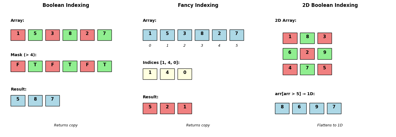
NumPy indexing extends beyond basic slicing to support boolean masks and integer arrays.
import numpy as np
import timeit

# Advanced indexing demonstration
data = np.arange(20).reshape(4, 5)
print("Original array:")
print(data)

# Boolean indexing
print("\nBoolean indexing (data > 10):")
mask = data > 10
print(f"Mask shape: {mask.shape}")
print(f"Result: {data[mask]}")  # Returns 1D array
print(f"Result shape: {data[mask].shape}")

# Fancy indexing with lists
print("\nFancy indexing with row selection:")
row_indices = [0, 2, 3]
selected_rows = data[row_indices]
print(f"Selected rows {row_indices}:")
print(selected_rows)

# 2D fancy indexing
print("\nFancy indexing for specific elements:")
rows = [0, 1, 2]
cols = [1, 3, 4]
elements = data[rows, cols]  # Selects (0,1), (1,3), (2,4)
print(f"Elements at (0,1), (1,3), (2,4): {elements}")

# Mixed indexing
print("\nMixed indexing (slice + fancy):")
mixed = data[:, [1, 3]]  # All rows, columns 1 and 3
print(mixed)

# Where function for conditional selection
print("\nUsing np.where for conditional operations:")
result = np.where(data > 10, data, 0)  # Replace values ≤10 with 0
print("Values > 10 kept, others become 0:")
print(result)

# Performance analysis
def compare_indexing_performance():
    """Compare different indexing approaches."""
    size = 100000
    arr = np.random.randint(0, 100, size)

    # Boolean indexing
    t_boolean = timeit.timeit(
        lambda: arr[arr > 50],
        number=100
    )

    # Fancy indexing
    indices = np.where(arr > 50)[0]
    t_fancy = timeit.timeit(
        lambda: arr[indices],
        number=100
    )

    # Basic slicing (for comparison)
    t_slice = timeit.timeit(
        lambda: arr[10000:20000],
        number=100
    )

    return t_boolean, t_fancy, t_slice

t_bool, t_fancy, t_slice = compare_indexing_performance()

print(f"\nIndexing performance (100,000 elements, 100 iterations):")
print(f"  Basic slicing: {t_slice:.3f}s (creates view)")
print(f"  Boolean indexing: {t_bool:.3f}s ({t_bool/t_slice:.0f}x slower)")
print(f"  Fancy indexing: {t_fancy:.3f}s ({t_fancy/t_slice:.0f}x slower)")

# Memory implications
large_array = np.random.rand(10000, 1000)
bool_mask = large_array > 0.5

print(f"\nMemory implications:")
print(f"  Original array: {large_array.nbytes / 1024**2:.1f} MB")
print(f"  Boolean mask: {bool_mask.nbytes / 1024**2:.1f} MB")
print(f"  Boolean result: {large_array[bool_mask].nbytes / 1024**2:.1f} MB")

# Advanced boolean operations
print(f"\nComplex boolean operations:")
arr = np.random.randint(0, 20, (5, 5))
print("Array:")
print(arr)

# Multiple conditions
complex_mask = (arr > 5) & (arr < 15)  # Element-wise AND
print(f"\nElements between 5 and 15: {arr[complex_mask]}")

# Any/all operations
print(f"Any element > 15: {np.any(arr > 15)}")
print(f"All elements > 0: {np.all(arr > 0)}")

# Axis-specific operations
print(f"Rows with any element > 15: {np.any(arr > 15, axis=1)}")
print(f"Columns with all elements > 5: {np.all(arr > 5, axis=0)}")
Original array:
[[ 0  1  2  3  4]
 [ 5  6  7  8  9]
 [10 11 12 13 14]
 [15 16 17 18 19]]

Boolean indexing (data > 10):
Mask shape: (4, 5)
Result: [11 12 13 14 15 16 17 18 19]
Result shape: (9,)

Fancy indexing with row selection:
Selected rows [0, 2, 3]:
[[ 0  1  2  3  4]
 [10 11 12 13 14]
 [15 16 17 18 19]]

Fancy indexing for specific elements:
Elements at (0,1), (1,3), (2,4): [ 1  8 14]

Mixed indexing (slice + fancy):
[[ 1  3]
 [ 6  8]
 [11 13]
 [16 18]]

Using np.where for conditional operations:
Values > 10 kept, others become 0:
[[ 0  0  0  0  0]
 [ 0  0  0  0  0]
 [ 0 11 12 13 14]
 [15 16 17 18 19]]

Indexing performance (100,000 elements, 100 iterations):
  Basic slicing: 0.000s (creates view)
  Boolean indexing: 0.026s (4109x slower)
  Fancy indexing: 0.002s (318x slower)

Memory implications:
  Original array: 76.3 MB
  Boolean mask: 9.5 MB
  Boolean result: 38.2 MB

Complex boolean operations:
Array:
[[ 5  0 14  2  6]
 [19  5  8  0  8]
 [15 13  3  1 12]
 [ 5  2 11  5 19]
 [17  4 14  9  8]]

Elements between 5 and 15: [14  6  8  8 13 12 11 14  9  8]
Any element > 15: True
All elements > 0: False
Rows with any element > 15: [False  True False  True  True]
Columns with all elements > 5: [False False False False  True]
Indexing creates views vs copies:
- Basic slicing: Creates views (shares memory)
- Boolean indexing: Always creates copies
- Fancy indexing: Always creates copies
- Views are faster but copies are safer
Pseudorandom Number Generation
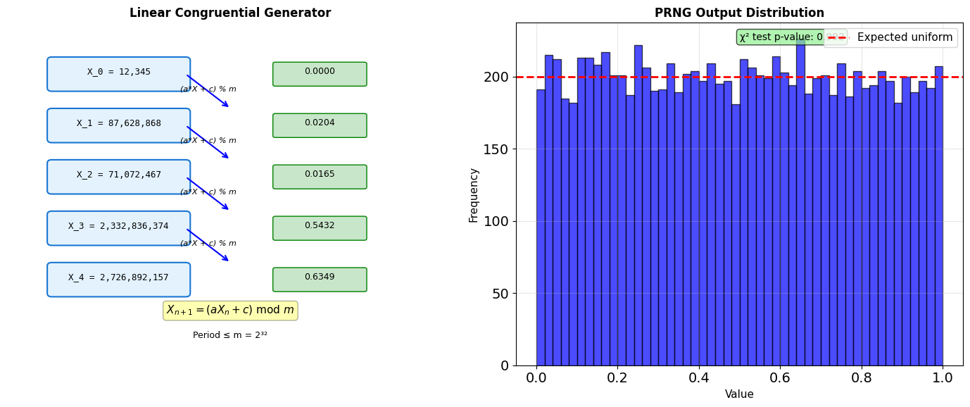
LCG (Linear Congruential Generator):
\[X_{n+1} = (aX_n + c) \mod m\]
- Simple, fast, but limited period (≤ m)
- Used historically; now superseded
Modern generator properties:
- Period: MT19937 has period 2^19937-1
- Quality: Pass TestU01 BigCrush (160 statistical tests)
- Speed: PCG64 is faster than MT19937
- State size: PCG64 uses 128 bits vs MT’s 19937 bits
PRNG output is deterministic given the seed — this enables reproducibility.
# Modern generators comparison
import numpy as np
import time

# Different PRNG algorithms
generators = {
    'PCG64': np.random.PCG64,
    'MT19937': np.random.MT19937,  # Mersenne Twister
    'Philox': np.random.Philox,
    'SFC64': np.random.SFC64,
}

print("Generator properties:")
for name, gen_class in generators.items():
    gen = np.random.Generator(gen_class(seed=42))

    # Generate samples for timing
    start = time.perf_counter()
    samples = gen.random(1000000)
    elapsed = time.perf_counter() - start

    print(f"\n{name}:")
    print(f"  Time for 1M: {elapsed:.3f}s")
    print(f"  Mean: {samples.mean():.6f}")
    print(f"  Std:  {samples.std():.6f}")

# State size comparison
mt = np.random.MT19937(seed=42)
pcg = np.random.PCG64(seed=42)

print(f"\nState size:")
print(f"  MT19937: {len(mt.state['state']['key'])} × 32 bits")
print(f"  PCG64: 2 × 64 bits")
Generator properties:
PCG64:
Time for 1M: 0.003s
Mean: 0.500026
Std: 0.288635
MT19937:
Time for 1M: 0.002s
Mean: 0.499778
Std: 0.288707
Philox:
Time for 1M: 0.003s
Mean: 0.499806
Std: 0.288525
SFC64:
Time for 1M: 0.003s
Mean: 0.499989
Std: 0.288734
State size:
MT19937: 624 × 32 bits
PCG64: 2 × 64 bits
NumPy Random Architecture
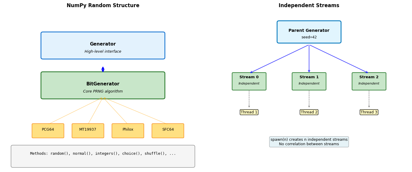
import numpy as np # Modern NumPy random (v1.17+) rng = np.random.default_rng(seed=42) # Basic generation print("Uniform [0, 1):", rng.random(5)) print("Integers [0, 10):", rng.integers(0, 10, size=5)) print("Normal(0, 1):", rng.normal(0, 1, size=5)) # Generator state management initial_state = rng.bit_generator.state # Generate some numbers vals1 = rng.random(3) print(f"\nFirst draw: {vals1}") # Restore state rng.bit_generator.state = initial_state vals2 = rng.random(3) print(f"After restore: {vals2}") print(f"Same values: {np.array_equal(vals1, vals2)}") # Spawn independent streams parent_rng = np.random.default_rng(seed=42) child_rngs = parent_rng.spawn(3) print("\nIndependent streams:") for i, child in enumerate(child_rngs): print(f" Stream {i}: {child.random(3)}")
Uniform [0, 1): [0.77395605 0.43887844 0.85859792 0.69736803 0.09417735]
Integers [0, 10): [5 9 7 7 7]
Normal(0, 1): [-0.01680116 -0.85304393 0.87939797 0.77779194 0.0660307 ]
First draw: [0.82276161 0.4434142 0.22723872]
After restore: [0.82276161 0.4434142 0.22723872]
Same values: True
Independent streams:
Stream 0: [0.91674416 0.91098667 0.8765925 ]
Stream 1: [0.46749078 0.0464489 0.59551001]
Stream 2: [0.0712392 0.71015972 0.07180046]
# Performance: vectorized vs loop import time rng = np.random.default_rng(seed=42) n = 1000000 # Vectorized generation start = time.perf_counter() vec_samples = rng.normal(0, 1, size=n) vec_time = time.perf_counter() - start # Loop generation start = time.perf_counter() loop_samples = [rng.normal(0, 1) for _ in range(n)] loop_time = time.perf_counter() - start print(f"Generation of {n:,} normals:") print(f" Vectorized: {vec_time:.3f}s") print(f" Loop: {loop_time:.3f}s") print(f" Speedup: {loop_time/vec_time:.1f}x") # Memory layout matters print(f"\nMemory layout:") print(f" Vectorized: {vec_samples.flags['C_CONTIGUOUS']}") print(f" Array strides: {vec_samples.strides}") # Custom distribution via inverse transform def exponential_inverse_transform(rng, rate, size): """Generate exponential via inverse CDF.""" u = rng.random(size) return -np.log(1 - u) / rate custom_exp = exponential_inverse_transform(rng, rate=2.0, size=1000) numpy_exp = rng.exponential(scale=0.5, size=1000) print(f"\nCustom vs NumPy exponential:") print(f" Custom mean: {custom_exp.mean():.3f}") print(f" NumPy mean: {numpy_exp.mean():.3f}") print(f" Theoretical: {0.5:.3f}")
Generation of 1,000,000 normals:
Vectorized: 0.004s
Loop: 0.311s
Speedup: 79.6x
Memory layout:
Vectorized: True
Array strides: (8,)
Custom vs NumPy exponential:
Custom mean: 0.507
NumPy mean: 0.497
Theoretical: 0.500
Distribution Sampling
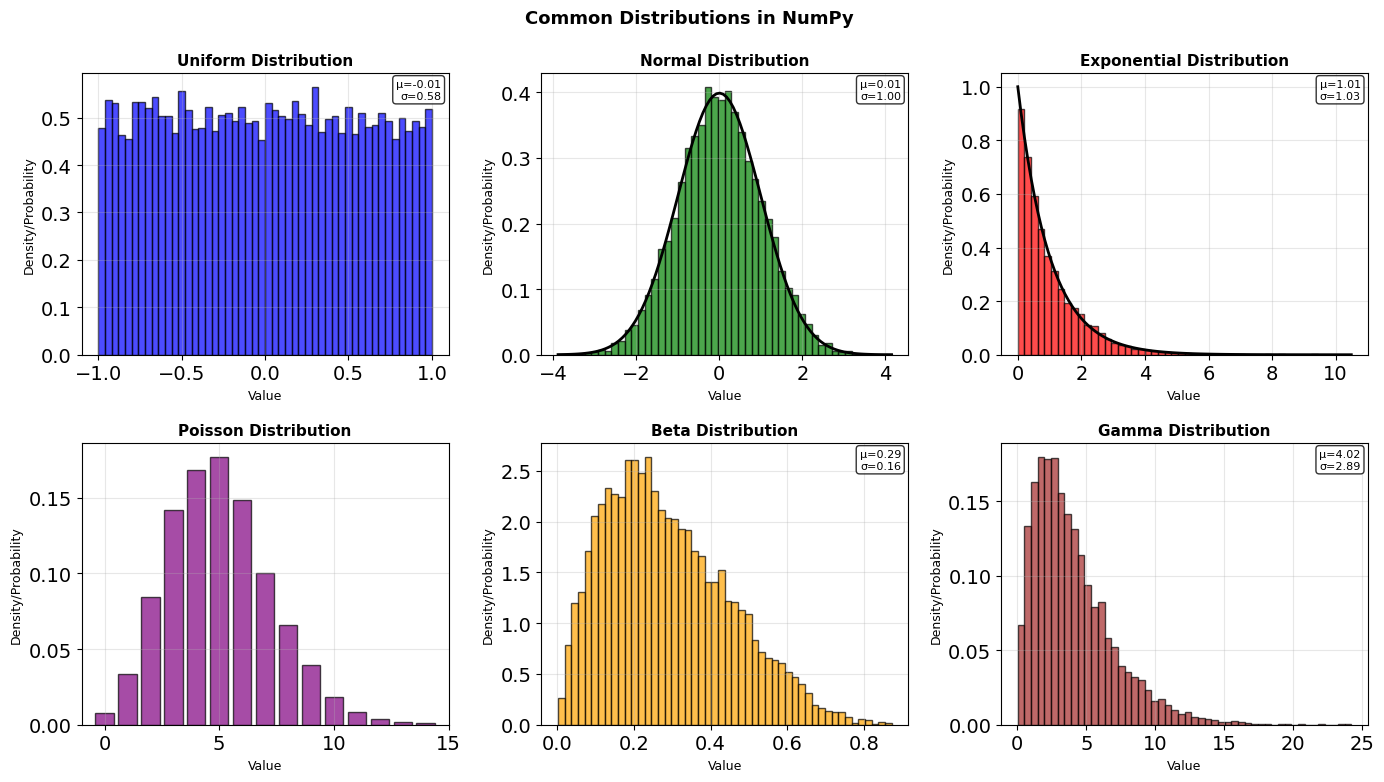
import numpy as np from scipy import stats rng = np.random.default_rng(seed=42) # Sampling from various distributions n = 1000 # Continuous distributions uniform = rng.uniform(low=0, high=10, size=n) normal = rng.normal(loc=100, scale=15, size=n) exponential = rng.exponential(scale=2.0, size=n) gamma = rng.gamma(shape=2, scale=2, size=n) # Discrete distributions poisson = rng.poisson(lam=3, size=n) binomial = rng.binomial(n=10, p=0.3, size=n) print("Sample statistics:") print(f"Uniform[0,10]: μ={uniform.mean():.2f}, σ={uniform.std():.2f}") print(f"Normal(100,15): μ={normal.mean():.2f}, σ={normal.std():.2f}") print(f"Exponential(2): μ={exponential.mean():.2f}, σ={exponential.std():.2f}") print(f"Poisson(3): μ={poisson.mean():.2f}, σ={poisson.std():.2f}") # Multivariate distributions mean = [0, 0] cov = [[1, 0.5], [0.5, 1]] multivariate = rng.multivariate_normal(mean, cov, size=1000) print(f"\nMultivariate normal:") print(f" Shape: {multivariate.shape}") print(f" Correlation: {np.corrcoef(multivariate.T)[0,1]:.3f}")
Sample statistics:
Uniform[0,10]: μ=4.97, σ=2.91
Normal(100,15): μ=98.83, σ=15.21
Exponential(2): μ=1.97, σ=1.96
Poisson(3): μ=2.97, σ=1.75
Multivariate normal:
Shape: (1000, 2)
Correlation: 0.459
# Transformation methods rng = np.random.default_rng(seed=42) # Box-Muller transform for normal def box_muller(rng, size): """Generate normal(0,1) from uniform.""" u1 = rng.random(size) u2 = rng.random(size) z0 = np.sqrt(-2 * np.log(u1)) * np.cos(2 * np.pi * u2) z1 = np.sqrt(-2 * np.log(u1)) * np.sin(2 * np.pi * u2) return z0, z1 z0, z1 = box_muller(rng, 5000) print(f"Box-Muller normal:") print(f" Mean: {z0.mean():.3f}, {z1.mean():.3f}") print(f" Std: {z0.std():.3f}, {z1.std():.3f}") # Rejection sampling for arbitrary distribution def rejection_sample(pdf, bounds, rng, n_samples): """Sample from arbitrary PDF via rejection.""" samples = [] low, high = bounds # Find maximum of PDF for efficiency x_test = np.linspace(low, high, 1000) max_pdf = np.max([pdf(x) for x in x_test]) while len(samples) < n_samples: x = rng.uniform(low, high) y = rng.uniform(0, max_pdf) if y <= pdf(x): samples.append(x) return np.array(samples) # Sample from beta-like distribution pdf = lambda x: 2 * x if 0 <= x <= 1 else 0 samples = rejection_sample(pdf, (0, 1), rng, 1000) print(f"\nRejection sampling:") print(f" Mean: {samples.mean():.3f} (theory: 0.667)")
Box-Muller normal:
Mean: -0.005, 0.000
Std: 1.002, 1.005
Rejection sampling:
Mean: 0.666 (theory: 0.667)
Monte Carlo Integration
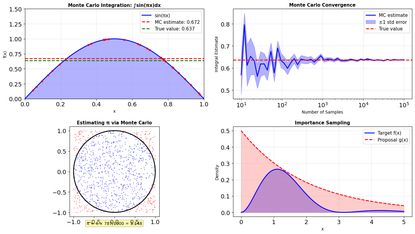
import numpy as np def monte_carlo_integrate(func, bounds, n_samples, rng=None): """Basic Monte Carlo integration.""" if rng is None: rng = np.random.default_rng() a, b = bounds # Sample uniformly in domain x = rng.uniform(a, b, n_samples) # Evaluate function y = func(x) # MC estimate: (b-a) * mean(f) integral = (b - a) * np.mean(y) std_error = (b - a) * np.std(y) / np.sqrt(n_samples) return integral, std_error # Example: ∫₀¹ sin(πx) dx = 2/π rng = np.random.default_rng(seed=42) for n in [100, 1000, 10000, 100000]: integral, error = monte_carlo_integrate( lambda x: np.sin(np.pi * x), bounds=(0, 1), n_samples=n, rng=rng ) true_value = 2/np.pi print(f"n={n:6d}: {integral:.5f} ± {error:.5f} (true: {true_value:.5f})") # Multidimensional integration def monte_carlo_nd(func, bounds, n_samples, rng=None): """N-dimensional Monte Carlo integration.""" if rng is None: rng = np.random.default_rng() ndim = len(bounds) volume = np.prod([b - a for a, b in bounds]) # Sample in hypercube samples = np.zeros((n_samples, ndim)) for i, (a, b) in enumerate(bounds): samples[:, i] = rng.uniform(a, b, n_samples) # Evaluate function values = np.array([func(*s) for s in samples]) integral = volume * np.mean(values) std_error = volume * np.std(values) / np.sqrt(n_samples) return integral, std_error # 2D example: ∫∫ exp(-(x²+y²)) dx dy over unit square def gaussian_2d(x, y): return np.exp(-(x**2 + y**2)) integral_2d, error_2d = monte_carlo_nd( gaussian_2d, bounds=[(0, 1), (0, 1)], n_samples=10000, rng=rng ) print(f"\n2D integral: {integral_2d:.5f} ± {error_2d:.5f}")
n= 100: 0.67226 ± 0.02825 (true: 0.63662)
n= 1000: 0.63032 ± 0.00972 (true: 0.63662)
n= 10000: 0.63801 ± 0.00308 (true: 0.63662)
n=100000: 0.63706 ± 0.00097 (true: 0.63662)
2D integral: 0.55976 ± 0.00217
# Variance reduction: stratified sampling def stratified_monte_carlo(func, bounds, n_strata, samples_per_stratum, rng=None): """Stratified Monte Carlo for variance reduction.""" if rng is None: rng = np.random.default_rng() a, b = bounds stratum_width = (b - a) / n_strata estimates = [] for i in range(n_strata): # Sample within stratum stratum_a = a + i * stratum_width stratum_b = a + (i + 1) * stratum_width x = rng.uniform(stratum_a, stratum_b, samples_per_stratum) y = func(x) # Stratum estimate estimates.append(np.mean(y)) # Combine strata integral = (b - a) * np.mean(estimates) std_error = (b - a) * np.std(estimates) / np.sqrt(n_strata) return integral, std_error # Compare standard vs stratified n_total = 10000 # Standard MC standard_int, standard_err = monte_carlo_integrate( lambda x: np.sin(np.pi * x), bounds=(0, 1), n_samples=n_total, rng=rng ) # Stratified MC n_strata = 100 stratified_int, stratified_err = stratified_monte_carlo( lambda x: np.sin(np.pi * x), bounds=(0, 1), n_strata=n_strata, samples_per_stratum=n_total // n_strata, rng=rng ) print(f"Variance reduction comparison ({n_total} samples):") print(f" Standard: {standard_int:.5f} ± {standard_err:.5f}") print(f" Stratified: {stratified_int:.5f} ± {stratified_err:.5f}") print(f" Error reduction: {standard_err/stratified_err:.2f}x")
Variance reduction comparison (10000 samples):
Standard: 0.63776 ± 0.00306
Stratified: 0.63655 ± 0.03078
Error reduction: 0.10x
Random Walks and Stochastic Processes
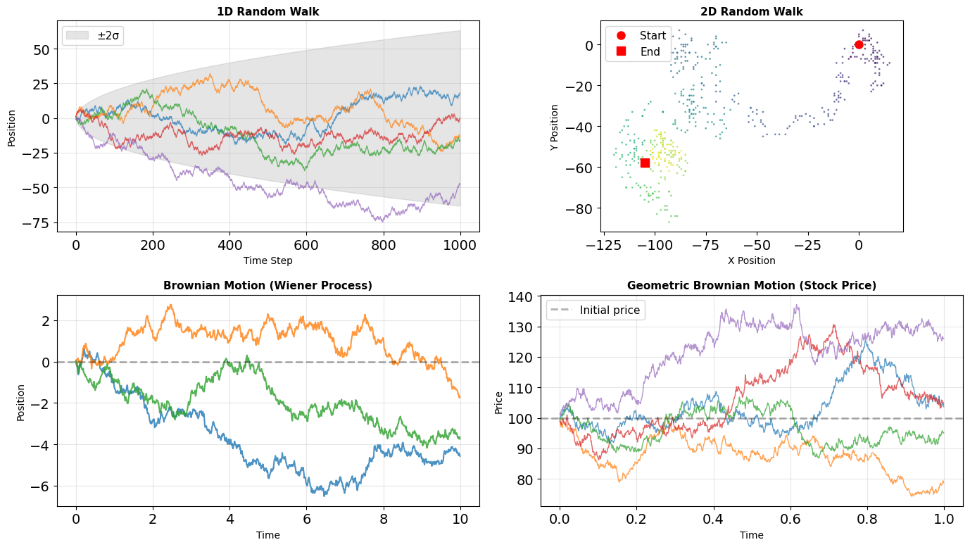
import numpy as np class RandomWalk: """1D and 2D random walk simulator.""" def __init__(self, seed=None): self.rng = np.random.default_rng(seed) def walk_1d(self, n_steps, p_up=0.5): """1D random walk with bias.""" steps = self.rng.choice( [-1, 1], size=n_steps, p=[1-p_up, p_up] ) return np.cumsum(steps) def walk_2d(self, n_steps): """2D random walk on lattice.""" # Possible moves: up, down, left, right moves = np.array([[0, 1], [0, -1], [-1, 0], [1, 0]]) choices = self.rng.integers(0, 4, size=n_steps) steps = moves[choices] path = np.cumsum(steps, axis=0) return path[:, 0], path[:, 1] def first_passage_time(self, barrier, max_steps=10000): """Time to first reach barrier.""" position = 0 for step in range(max_steps): position += self.rng.choice([-1, 1]) if abs(position) >= barrier: return step + 1 return None # Analyze random walk properties walker = RandomWalk(seed=42) # First passage times barriers = [10, 20, 50] n_trials = 1000 for barrier in barriers: times = [] for _ in range(n_trials): t = walker.first_passage_time(barrier) if t is not None: times.append(t) mean_time = np.mean(times) theoretical = barrier ** 2 # E[T] = n² for symmetric walk print(f"Barrier ±{barrier}:") print(f" Mean time: {mean_time:.1f}") print(f" Theory: {theoretical:.1f}") print(f" Success rate: {len(times)/n_trials:.1%}")
Barrier ±10:
Mean time: 99.2
Theory: 100.0
Success rate: 100.0%
Barrier ±20:
Mean time: 405.9
Theory: 400.0
Success rate: 100.0%
Barrier ±50:
Mean time: 2384.1
Theory: 2500.0
Success rate: 99.3%
# Stochastic differential equations def euler_maruyama(sde_drift, sde_diffusion, x0, t_span, dt, rng=None): """Solve SDE using Euler-Maruyama method.""" if rng is None: rng = np.random.default_rng() t = np.arange(t_span[0], t_span[1], dt) n = len(t) x = np.zeros(n) x[0] = x0 # Generate all random increments at once dW = rng.normal(0, np.sqrt(dt), n-1) for i in range(n-1): drift = sde_drift(x[i], t[i]) diffusion = sde_diffusion(x[i], t[i]) x[i+1] = x[i] + drift*dt + diffusion*dW[i] return t, x # Ornstein-Uhlenbeck process (mean-reverting) def ou_drift(x, t, theta=1.0, mu=0.0): return theta * (mu - x) def ou_diffusion(x, t, sigma=0.3): return sigma rng = np.random.default_rng(seed=42) # Simulate multiple paths print("Ornstein-Uhlenbeck process:") for x0 in [2.0, 0.0, -2.0]: t, x = euler_maruyama( ou_drift, ou_diffusion, x0=x0, t_span=(0, 10), dt=0.01, rng=rng ) print(f" Start: {x0:+.1f}, End: {x[-1]:+.2f}, Mean: {x[len(x)//2:].mean():+.2f}") # Geometric Brownian Motion def gbm_drift(S, t, mu=0.05): return mu * S def gbm_diffusion(S, t, sigma=0.2): return sigma * S t, S = euler_maruyama( gbm_drift, gbm_diffusion, x0=100, t_span=(0, 1), dt=0.001, rng=rng ) print(f"\nGBM Stock simulation:") print(f" Initial: ${S[0]:.2f}") print(f" Final: ${S[-1]:.2f}") print(f" Return: {(S[-1]/S[0] - 1)*100:.1f}%")
Ornstein-Uhlenbeck process:
Start: +2.0, End: +0.05, Mean: -0.15
Start: +0.0, End: -0.57, Mean: -0.38
Start: -2.0, End: +0.19, Mean: +0.13
GBM Stock simulation:
Initial: $100.00
Final: $104.77
Return: 4.8%
Reproducibility and Parallel Streams
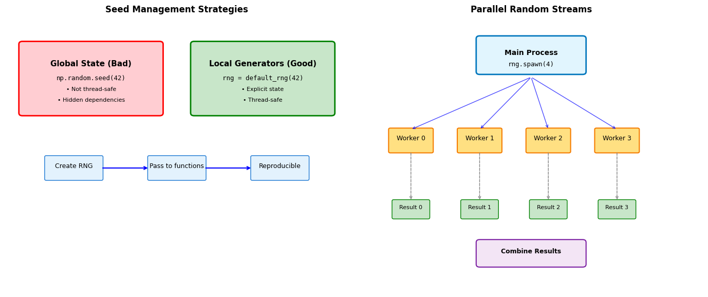
import numpy as np from concurrent.futures import ProcessPoolExecutor import multiprocessing as mp def monte_carlo_pi(n_samples, seed): """Estimate π using Monte Carlo.""" rng = np.random.default_rng(seed) # Generate points in unit square x = rng.random(n_samples) y = rng.random(n_samples) # Count points inside circle inside = (x**2 + y**2) <= 1 pi_estimate = 4 * inside.sum() / n_samples return pi_estimate # Serial execution rng_main = np.random.default_rng(seed=42) n_trials = 4 n_samples = 1000000 print("Serial execution:") serial_results = [] for i in range(n_trials): # Use different seed for each trial seed = rng_main.integers(0, 2**32) result = monte_carlo_pi(n_samples, seed) serial_results.append(result) print(f" Trial {i}: π ≈ {result:.5f}") print(f" Mean: {np.mean(serial_results):.5f}") print(f" Std: {np.std(serial_results):.5f}") # Parallel execution with spawned generators def parallel_monte_carlo(): """Parallel MC with independent streams.""" parent_rng = np.random.default_rng(seed=42) # Spawn independent streams n_workers = mp.cpu_count() child_seeds = parent_rng.spawn(n_workers) # Create tasks with independent seeds tasks = [] for i in range(n_workers): # Extract seed value from SeedSequence seed_value = child_seeds[i].generate_state(1)[0] tasks.append((n_samples, seed_value)) return tasks # Note: ProcessPoolExecutor not shown due to execution environment print(f"\nParallel setup for {mp.cpu_count()} cores created")
Serial execution:
Trial 0: π ≈ 3.14089
Trial 1: π ≈ 3.14045
Trial 2: π ≈ 3.14242
Trial 3: π ≈ 3.14100
Mean: 3.14119
Std: 0.00074
Parallel setup for 10 cores created
Reproducibility patterns:
# Use explicit generators (not global state) rng = np.random.default_rng(seed=42) # Pass rng to functions explicitly def simulate(n, rng): return rng.normal(0, 1, n) # Save/restore state for checkpoints state = rng.bit_generator.state # ... do work ... rng.bit_generator.state = state # restore # Use spawn() for parallel work children = rng.spawn(4) # 4 independent streams
Avoid:
np.random.seed()— global state, not thread-safe- Creating
default_rng()without seed inside loops
Same seed + same code = identical results.
Lambda Functions: Anonymous Functions in Python
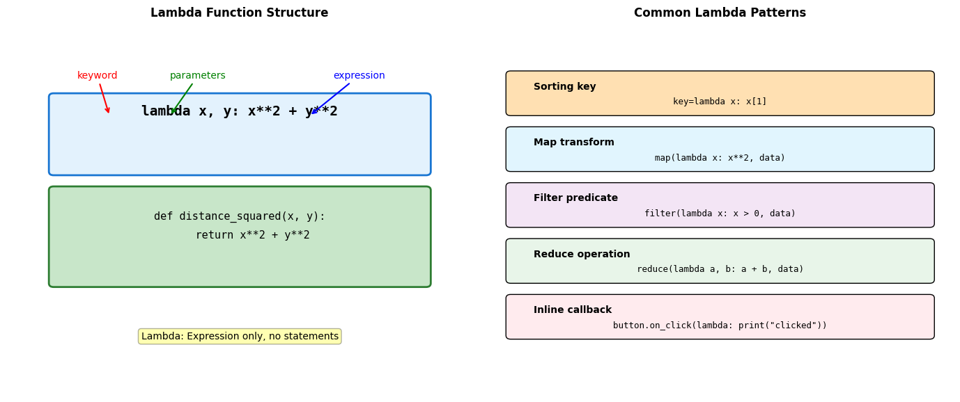
# Lambda basics square = lambda x: x**2 add = lambda x, y: x + y magnitude = lambda v: sum(x**2 for x in v) ** 0.5 print(f"square(5) = {square(5)}") print(f"add(3, 4) = {add(3, 4)}") print(f"magnitude([3, 4]) = {magnitude([3, 4])}") # Lambda limitations - no statements try: # This won't work - assignment is a statement bad_lambda = lambda x: (y := x + 1, y * 2) except SyntaxError as e: print(f"\nSyntax error in lambda") # Workaround using expression forms result = (lambda x: (x + 1) * 2)(5) print(f"Workaround result: {result}") # Lambda with conditional expression abs_val = lambda x: x if x >= 0 else -x sign = lambda x: 1 if x > 0 else (-1 if x < 0 else 0) print(f"\nabs_val(-5) = {abs_val(-5)}") print(f"sign(-5) = {sign(-5)}") print(f"sign(0) = {sign(0)}") print(f"sign(5) = {sign(5)}")
square(5) = 25
add(3, 4) = 7
magnitude([3, 4]) = 5.0
Workaround result: 12
abs_val(-5) = 5
sign(-5) = -1
sign(0) = 0
sign(5) = 1
# Lambdas in data processing import numpy as np # Sorting with custom key points = [(3, 4), (1, 2), (5, 1), (2, 3)] # Sort by distance from origin by_distance = sorted(points, key=lambda p: (p[0]**2 + p[1]**2)**0.5) print(f"By distance: {by_distance}") # Sort by second coordinate by_y = sorted(points, key=lambda p: p[1]) print(f"By y-coord: {by_y}") # Complex sorting - primary and secondary keys data = [('Alice', 85), ('Bob', 92), ('Charlie', 85), ('David', 78)] sorted_data = sorted(data, key=lambda x: (-x[1], x[0])) print(f"\nBy score desc, then name:") for name, score in sorted_data: print(f" {name}: {score}") # Lambda in numerical operations vectors = np.array([[1, 2], [3, 4], [5, 6]]) # Apply transformation transform = lambda v: v / np.linalg.norm(v) normalized = np.apply_along_axis(transform, 1, vectors) print(f"\nNormalized vectors:") print(normalized)
By distance: [(1, 2), (2, 3), (3, 4), (5, 1)]
By y-coord: [(5, 1), (1, 2), (2, 3), (3, 4)]
By score desc, then name:
Bob: 92
Alice: 85
Charlie: 85
David: 78
Normalized vectors:
[[0.4472136 0.89442719]
[0.6 0.8 ]
[0.6401844 0.76822128]]
Lambda Performance and Pitfalls
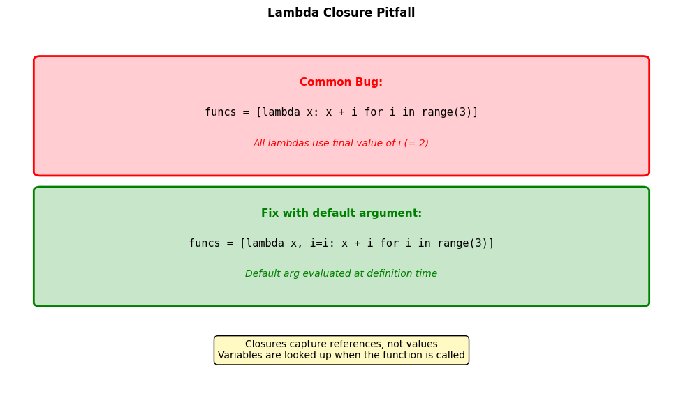
# Closure pitfall demonstration print("Closure problem:") funcs_bad = [] for i in range(3): funcs_bad.append(lambda x: x + i) # All functions use final value of i for j, f in enumerate(funcs_bad): print(f" func[{j}](10) = {f(10)}") # All return 12! print("\nFixed with default argument:") funcs_good = [] for i in range(3): funcs_good.append(lambda x, i=i: x + i) for j, f in enumerate(funcs_good): print(f" func[{j}](10) = {f(10)}") # Correct: 10, 11, 12 # Alternative: use functools.partial from functools import partial def add(x, y): return x + y print("\nUsing partial:") funcs_partial = [partial(add, y=i) for i in range(3)] for j, f in enumerate(funcs_partial): print(f" func[{j}](10) = {f(10)}")
Closure problem:
func[0](10) = 12
func[1](10) = 12
func[2](10) = 12
Fixed with default argument:
func[0](10) = 10
func[1](10) = 11
func[2](10) = 12
Using partial:
func[0](10) = 10
func[1](10) = 11
func[2](10) = 12
Closure capture rule:
Closures capture references to variables, not values. The variable is looked up when the function is called, not when it’s defined.
Fixes:
- Default argument:
lambda x, i=i: x + i functools.partial: binds value at creation time- Nested function with local binding
When lambdas are appropriate:
- Short, single-expression functions
- Throwaway functions for
sort,map,filter - Simple callbacks
Prefer named functions when:
- Logic is complex or reusable
- You need docstrings or type hints
- Debugging is important (lambdas have no name)
Map, Filter, Reduce: Functional Transformations
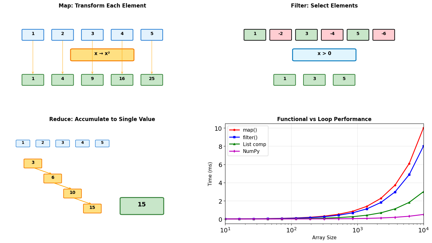
from functools import reduce import operator data = [1, 2, 3, 4, 5] # Map: transform each element squared = list(map(lambda x: x**2, data)) print(f"Original: {data}") print(f"Squared: {squared}") # Filter: select elements evens = list(filter(lambda x: x % 2 == 0, data)) odds = list(filter(lambda x: x % 2 == 1, data)) print(f"\nEvens: {evens}") print(f"Odds: {odds}") # Reduce: accumulate to single value sum_all = reduce(operator.add, data) product = reduce(operator.mul, data) max_val = reduce(lambda a, b: a if a > b else b, data) print(f"\nSum: {sum_all}") print(f"Product: {product}") print(f"Max: {max_val}") # Combining operations result = reduce( operator.add, filter( lambda x: x > 10, map(lambda x: x**2, data) ) ) print(f"\nSum of squares > 10: {result}") # Functional pipeline def pipeline(data, *functions): """Apply functions in sequence.""" for func in functions: data = func(data) return data result = pipeline( range(10), lambda x: map(lambda n: n**2, x), lambda x: filter(lambda n: n % 2 == 0, x), list ) print(f"\nPipeline result: {result}")
Original: [1, 2, 3, 4, 5]
Squared: [1, 4, 9, 16, 25]
Evens: [2, 4]
Odds: [1, 3, 5]
Sum: 15
Product: 120
Max: 5
Sum of squares > 10: 41
Pipeline result: [0, 4, 16, 36, 64]
# Performance comparison import timeit import numpy as np data = list(range(1000)) # Map alternatives t_map = timeit.timeit( lambda: list(map(lambda x: x**2, data)), number=1000 ) t_comp = timeit.timeit( lambda: [x**2 for x in data], number=1000 ) t_numpy = timeit.timeit( lambda: np.array(data)**2, number=1000 ) print(f"Squaring 1000 numbers:") print(f" map(): {t_map:.3f}s") print(f" List comp: {t_comp:.3f}s ({t_map/t_comp:.2f}x)") print(f" NumPy: {t_numpy:.3f}s ({t_map/t_numpy:.1f}x)") # Memory efficiency print(f"\nMemory behavior:") # Map returns iterator (lazy) mapped = map(lambda x: x**2, range(1000000)) print(f" map object: {sys.getsizeof(mapped)} bytes") # List comprehension creates full list comp = [x**2 for x in range(100000)] # Smaller for memory print(f" List comp (100k): {sys.getsizeof(comp):,} bytes") # Generator expression (lazy like map) gen = (x**2 for x in range(1000000)) print(f" Generator expr: {sys.getsizeof(gen)} bytes") # Practical reduce example from itertools import accumulate # Running statistics values = [3, 1, 4, 1, 5, 9, 2, 6] running_sum = list(accumulate(values)) running_max = list(accumulate(values, max)) print(f"\nValues: {values}") print(f"Running sum: {running_sum}") print(f"Running max: {running_max}")
Squaring 1000 numbers:
map(): 0.028s
List comp: 0.017s (1.67x)
NumPy: 0.025s (1.1x)
Memory behavior:
map object: 48 bytes
List comp (100k): 800,984 bytes
Generator expr: 200 bytes
Values: [3, 1, 4, 1, 5, 9, 2, 6]
Running sum: [3, 4, 8, 9, 14, 23, 25, 31]
Running max: [3, 3, 4, 4, 5, 9, 9, 9]
Map, Filter, Reduce in Numerical Computing
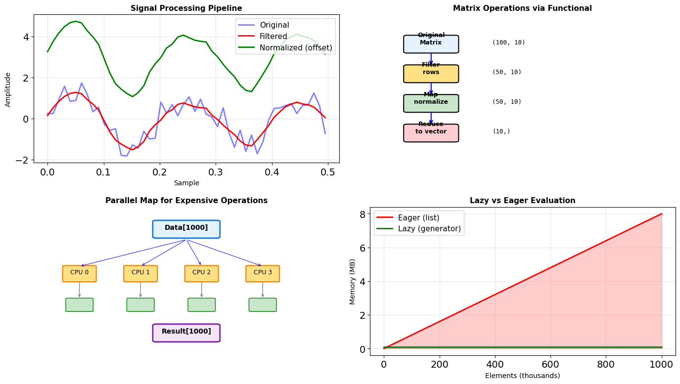
import numpy as np from functools import reduce # Signal processing pipeline def process_signals(signals): """Functional signal processing pipeline.""" # Filter: remove invalid signals valid = filter(lambda s: not np.any(np.isnan(s)), signals) # Map: normalize each signal normalized = map(lambda s: (s - s.mean()) / s.std(), valid) # Map: compute features features = map(lambda s: { 'energy': np.sum(s**2), 'peak': np.max(np.abs(s)), 'zero_crossings': np.sum(np.diff(np.sign(s)) != 0) }, normalized) return list(features) # Generate test signals np.random.seed(42) signals = [ np.sin(np.linspace(0, 2*np.pi, 100)) + 0.1*np.random.randn(100), np.random.randn(100), np.array([np.nan] * 100), # Invalid np.cos(np.linspace(0, 4*np.pi, 100)), ] results = process_signals(signals) print("Signal features:") for i, feat in enumerate(results): print(f" Signal {i}: energy={feat['energy']:.1f}, " f"peak={feat['peak']:.2f}, crossings={feat['zero_crossings']}") # Matrix operations with functional approach def matrix_pipeline(matrix): """Process matrix rows functionally.""" # Filter rows by condition filtered_rows = filter( lambda row: np.sum(row) > 0, matrix ) # Normalize each row normalized = map( lambda row: row / np.linalg.norm(row), filtered_rows ) # Reduce to summary statistics row_list = list(normalized) if row_list: mean_row = reduce( lambda a, b: a + b, row_list ) / len(row_list) return mean_row return None # Test matrix matrix = np.random.randn(10, 5) matrix[2] = -np.abs(matrix[2]) # Make one row negative sum result = matrix_pipeline(matrix) print(f"\nMean normalized row: {result}")
Signal features:
Signal 0: energy=100.0, peak=1.80, crossings=3
Signal 1: energy=100.0, peak=2.84, crossings=54
Signal 2: energy=100.0, peak=1.42, crossings=4
Mean normalized row: [ 0.01159341 0.05561288 -0.05330941 0.1654067 0.35741119]
# Parallel map for expensive operations from multiprocessing import Pool import time def expensive_computation(x): """Simulate expensive computation.""" # In real code, this might be optimization, simulation, etc. result = 0 for i in range(100000): result += x * np.sin(i) * np.cos(i) return result / 100000 # Sequential map data = list(range(10)) start = time.perf_counter() sequential_results = list(map(expensive_computation, data)) seq_time = time.perf_counter() - start print(f"Sequential map: {seq_time:.3f}s") # Parallel map (simplified for demonstration) # Note: In Jupyter/interactive environments, use: # from multiprocessing.dummy import Pool # Thread pool # Or restructure for subprocess pool def parallel_map(func, data, n_workers=4): """Simple parallel map implementation.""" # Simulate parallel execution # In production, use multiprocessing.Pool results = [] chunk_size = len(data) // n_workers for i in range(0, len(data), chunk_size): chunk = data[i:i+chunk_size] results.extend(map(func, chunk)) return results # Lazy evaluation for large datasets def lazy_pipeline(data_generator): """Process infinite/large data streams.""" # Chain of transformations (all lazy) transformed = map(lambda x: x**2, data_generator) filtered = filter(lambda x: x % 2 == 0, transformed) processed = map(lambda x: x // 2, filtered) # Only compute what's needed return processed # Infinite generator def fibonacci(): a, b = 0, 1 while True: yield a a, b = b, a + b # Process only first 10 values pipeline = lazy_pipeline(fibonacci()) first_10 = [next(pipeline) for _ in range(10)] print(f"\nFirst 10 processed Fibonacci: {first_10}") # Memory comparison import sys eager_list = [x**2 for x in range(100000)] lazy_gen = (x**2 for x in range(100000)) print(f"\nMemory usage:") print(f" Eager list: {sys.getsizeof(eager_list):,} bytes") print(f" Lazy generator: {sys.getsizeof(lazy_gen):,} bytes")
Sequential map: 0.821s
First 10 processed Fibonacci: [0, 2, 32, 578, 10368, 186050, 3338528, 59907458, 1074995712, 19290015362]
Memory usage:
Eager list: 800,984 bytes
Lazy generator: 200 bytes
Partial Functions and Currying
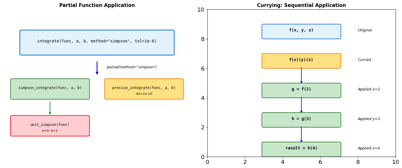
from functools import partial, reduce import operator # Partial function application def power(base, exponent): return base ** exponent # Create specialized functions square = partial(power, exponent=2) cube = partial(power, exponent=3) two_to_power = partial(power, base=2) # 2^x print("Partial functions:") print(f" square(5) = {square(5)}") print(f" cube(5) = {cube(5)}") print(f" 2^10 = {two_to_power(exponent=10)}") # Partial with multiple arguments def integrate(func, lower, upper, method='trapezoid', n_points=100): """Numerical integration.""" x = np.linspace(lower, upper, n_points) y = func(x) if method == 'trapezoid': return np.trapezoid(y, x) elif method == 'simpson': from scipy.integrate import simpson return simpson(y, x=x) else: raise ValueError(f"Unknown method: {method}") # Create specialized integrators simpson_integrate = partial(integrate, method='simpson') unit_integrate = partial(integrate, lower=0, upper=1) precise_integrate = partial(integrate, n_points=1000) # Use specialized versions result1 = simpson_integrate(np.sin, 0, np.pi) result2 = unit_integrate(lambda x: x**2) result3 = precise_integrate(np.exp, 0, 1) print(f"\nIntegration results:") print(f" ∫sin(x)dx [0,π] = {result1:.4f}") print(f" ∫x²dx [0,1] = {result2:.4f}") print(f" ∫e^x dx [0,1] = {result3:.4f}")
Partial functions:
square(5) = 25
cube(5) = 125
2^10 = 1024
Integration results:
∫sin(x)dx [0,π] = 2.0000
∫x²dx [0,1] = 0.3334
∫e^x dx [0,1] = 1.7183
functools.partial use cases:
- Pre-filling arguments for callbacks
- Creating specialized versions of general functions
- Configuration injection (default parameters)
# Common pattern: create specialized functions from functools import partial # Pre-configured logger debug_log = partial(print, "[DEBUG]") error_log = partial(print, "[ERROR]") # Pre-configured numerical operations normalize = partial(np.divide, b=255.0) clip_unit = partial(np.clip, a_min=0, a_max=1)
Currying (sequential application) is less common in Python than in functional languages. Use partial instead — it’s explicit and readable.
Composition pattern:
def compose(*funcs): """Compose functions: compose(f, g)(x) = f(g(x))""" return reduce(lambda f, g: lambda x: f(g(x)), funcs)
Decorators for Instrumentation
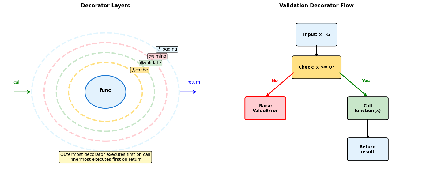
import time import functools def timer(func): """Simple timing decorator.""" @functools.wraps(func) def wrapper(*args, **kwargs): start = time.perf_counter() result = func(*args, **kwargs) elapsed = time.perf_counter() - start print(f"{func.__name__} took {elapsed:.4f}s") return result return wrapper @timer def compute_sum(n): """Sum integers from 0 to n.""" return sum(range(n)) # Use decorated function result = compute_sum(1000000) print(f"Result: {result}") # Decorator with arguments (decorator factory) def repeat(n_times): """Decorator factory: repeat function call.""" def decorator(func): @functools.wraps(func) def wrapper(*args, **kwargs): results = [] for _ in range(n_times): results.append(func(*args, **kwargs)) return results return wrapper return decorator @repeat(3) def random_number(): import random return random.random() print(f"\nThree random numbers: {random_number()}")
compute_sum took 0.0063s
Result: 499999500000
Three random numbers: [0.587228135960648, 0.9059035195407342, 0.6639487938573434]
Decorator pattern:
@decorator def func(): pass # Equivalent to: func = decorator(func)
Use functools.wraps to preserve the original function’s metadata (__name__, __doc__).
Common decorator uses:
- Timing/profiling
- Logging
- Caching (
@functools.lru_cache) - Validation
- Authentication/authorization
Decorator factory (decorator with arguments):
@factory(arg) # factory(arg) returns decorator def func(): pass # Equivalent to: func = factory(arg)(func)
Stacking decorators:
@dec1 @dec2 def func(): pass # Equivalent to: func = dec1(dec2(func)) # dec2 wraps func first, then dec1 wraps that
SciPy Architecture: Python Interface to Fortran/C Libraries
SciPy provides Python bindings to decades of optimized numerical code.
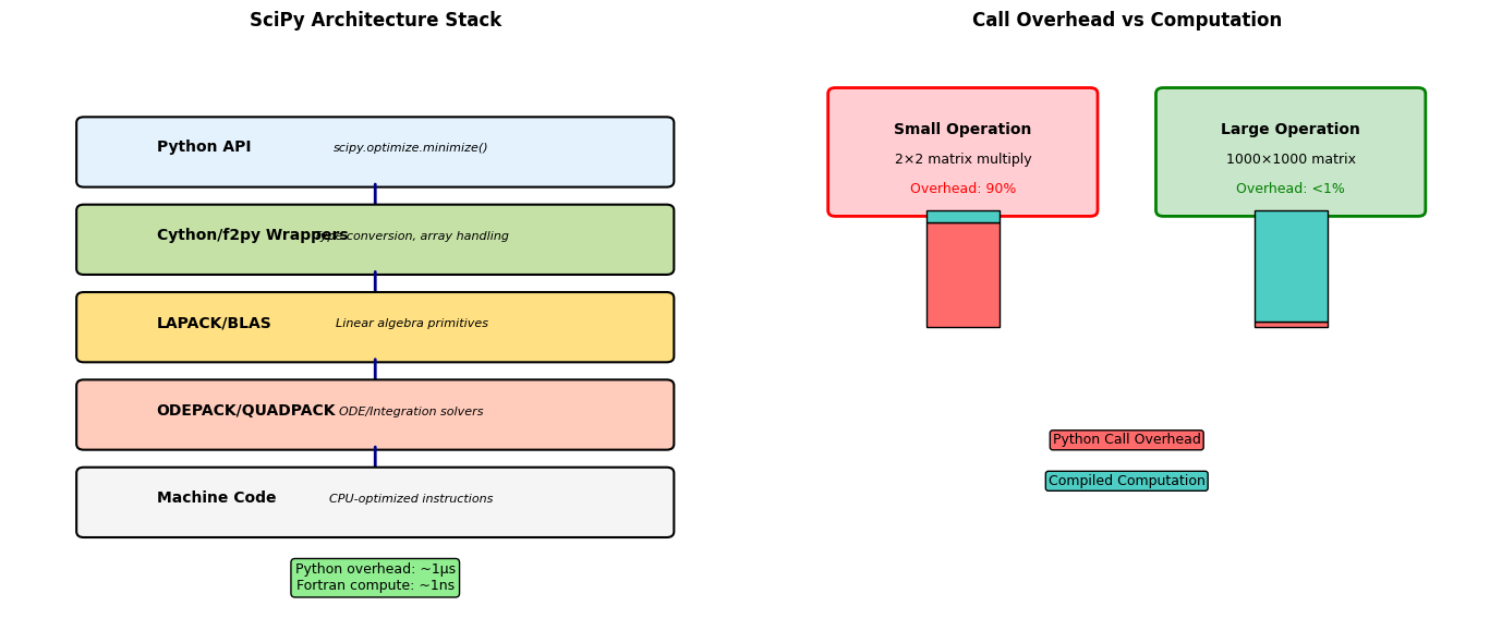
import scipy import numpy as np import timeit # Demonstrate overhead vs computation def small_operation(): """Python function call dominates.""" A = np.array([[1, 2], [3, 4]]) return scipy.linalg.inv(A) def large_operation(): """Fortran computation dominates.""" A = np.random.randn(1000, 1000) return scipy.linalg.inv(A) # Measure call overhead empty_call = timeit.timeit(lambda: None, number=100000) print(f"Python function call: {empty_call*10:.2f}μs") # Small vs large operation efficiency A_small = np.random.randn(2, 2) A_large = np.random.randn(100, 100) t_small = timeit.timeit( lambda: scipy.linalg.inv(A_small), number=10000 ) t_large = timeit.timeit( lambda: scipy.linalg.inv(A_large), number=100 ) print(f"\n2×2 inversion: {t_small/10:.1f}μs per call") print(f"100×100 inversion: {t_large*10:.1f}ms per call") # BLAS level comparison flops_small = 2**3 # O(n³) for inversion flops_large = 100**3 print(f"\nFLOPS ratio: {flops_large/flops_small:,.0f}×") print(f"Time ratio: {(t_large/100)/(t_small/10000):.0f}×") print(f"Efficiency gain: {(flops_large/flops_small)/((t_large/100)/(t_small/10000)):.1f}×")
Python function call: 0.01μs
2×2 inversion: 0.0μs per call
100×100 inversion: 0.1ms per call
FLOPS ratio: 125,000×
Time ratio: 38×
Efficiency gain: 3280.7×
Design Implications:
-
Wrapper overhead is constant - Same Python call cost regardless of problem size
-
Amortization strategy - Process vectors/matrices, not scalars
-
Library selection hierarchy:
- Intel MKL (commercial, fastest)
- OpenBLAS (open source, competitive)
- Reference BLAS (portable, slow)
-
Memory layout matters - Fortran order (column-major) vs C order (row-major)
# SciPy provides optimized numerical routines print(f"SciPy version: {scipy.__version__}") print(f"Available submodules: {len([m for m in dir(scipy) if not m.startswith('_')])}")
SciPy version: 1.17.1
Available submodules: 21
Optimization: Interior Point vs Simplex Methods
Different algorithms excel at different problem structures.
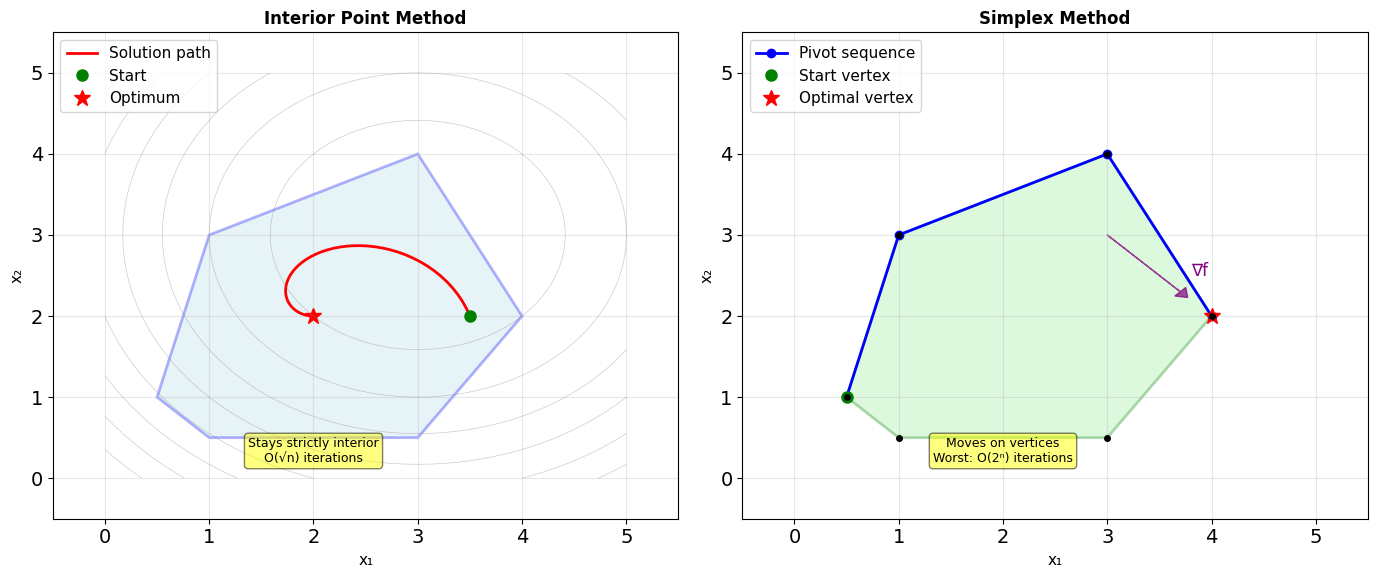
from scipy.optimize import linprog import numpy as np # Linear programming problem: # minimize: -x - 2y # subject to: x + 2y <= 8 # 2x + y <= 8 # x, y >= 0 c = [-1, -2] # Coefficients (minimize) A_ub = [[1, 2], [2, 1]] # Inequality constraints b_ub = [8, 8] bounds = [(0, None), (0, None)] # Compare methods methods = ['interior-point', 'simplex', 'highs'] for method in methods: result = linprog(c, A_ub=A_ub, b_ub=b_ub, bounds=bounds, method=method) print(f"{method:15s}: x={result.x}, " f"iterations={result.nit}") # Performance characteristics n_vars = [10, 100, 1000] for n in n_vars: # Random LP problem c = np.random.randn(n) A = np.random.randn(n//2, n) b = np.random.randn(n//2) import time # Interior point start = time.perf_counter() res_ip = linprog(c, A_ub=A, b_ub=b, method='interior-point', options={'disp': False}) time_ip = time.perf_counter() - start # Simplex start = time.perf_counter() res_simplex = linprog(c, A_ub=A, b_ub=b, method='simplex', options={'disp': False}) time_simplex = time.perf_counter() - start print(f"\nn={n:4d} variables:") print(f" Interior: {time_ip*1000:6.1f}ms") print(f" Simplex: {time_simplex*1000:6.1f}ms")
interior-point : x=[1.69596234 3.15201883], iterations=4
simplex : x=[2.66666667 2.66666667], iterations=2
highs : x=[0. 4.], iterations=2
n= 10 variables:
Interior: 0.8ms
Simplex: 0.7ms
n= 100 variables:
Interior: 1.0ms
Simplex: 14.5ms
n=1000 variables:
Interior: 26.8ms
Simplex: 817.9ms
Algorithm Selection Criteria:
Interior Point:
- Polynomial worst-case: O(n³·⁵)
- Better for large, dense problems
- Generates strictly feasible iterates
- Smooth convergence profile
Simplex:
- Exponential worst-case, excellent average-case
- Superior for sparse problems
- Always at a vertex (basic feasible solution)
- Can exploit problem structure
Modern hybrids (HiGHS):
- Crossover between methods
- Presolver eliminates variables
- Parallel execution paths
Root Finding: Convergence Rates and Stability
Root finding methods trade convergence speed for robustness.
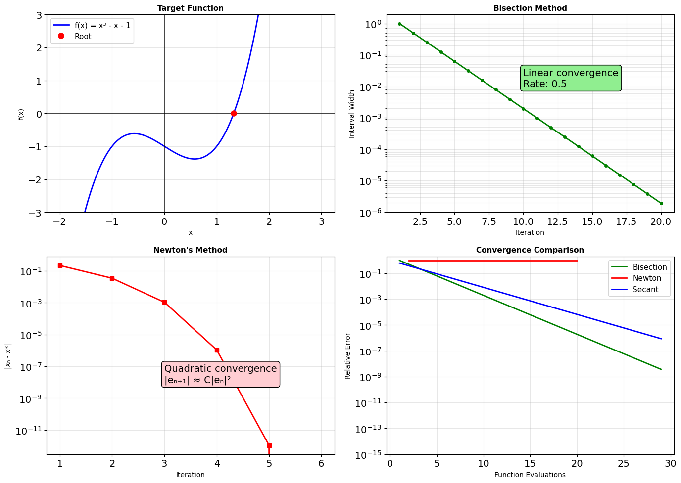
from scipy import optimize import numpy as np def f(x): """Test function with known root.""" return x**3 - x - 1 def fprime(x): """Derivative of f.""" return 3*x**2 - 1 # Compare root finding methods x0 = 2.0 # Initial guess bracket = [1, 2] # Known bracket # Bisection: guaranteed convergence root_bisect = optimize.bisect(f, *bracket) print(f"Bisection: {root_bisect:.10f}") # Brent: combines bisection, secant, inverse quadratic root_brent = optimize.brentq(f, *bracket) print(f"Brent: {root_brent:.10f}") # Newton: fast but needs derivative root_newton = optimize.newton(f, x0, fprime=fprime) print(f"Newton: {root_newton:.10f}") # Performance comparison import timeit n = 1000 times = {} times['bisect'] = timeit.timeit( lambda: optimize.bisect(f, 1, 2), number=n ) times['brent'] = timeit.timeit( lambda: optimize.brentq(f, 1, 2), number=n ) times['newton'] = timeit.timeit( lambda: optimize.newton(f, 2.0, fprime=fprime), number=n ) print(f"\nTime for {n} root findings:") for method, time in times.items(): print(f" {method:8s}: {time*1000:.1f}ms")
Bisection: 1.3247179572
Brent: 1.3247179572
Newton: 1.3247179572
Time for 1000 root findings:
bisect : 16.2ms
brent : 4.5ms
newton : 37.7ms
Method Characteristics:
Bisection:
- Requires bracket [a, b] where f(a)·f(b) < 0
- Guaranteed convergence
- Linear rate: log₂(ε₀/ε) iterations
- One function evaluation per iteration
Newton-Raphson:
- Requires derivative
- Quadratic convergence near root
- Can diverge or cycle
- Two evaluations per iteration (f and f’)
Brent’s Method (scipy default):
- Hybrid: bisection + secant + inverse quadratic
- Guaranteed convergence with bracket
- Superlinear convergence in practice
- Adaptive algorithm selection
Numerical Integration: Adaptive Quadrature
Integration routines balance function evaluations against accuracy.
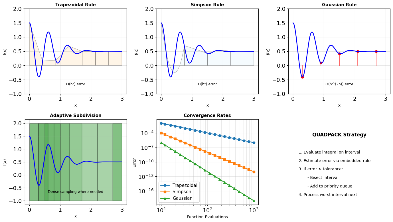
from scipy import integrate import numpy as np def oscillatory(x): """Challenging integrand.""" return np.exp(-x**2) * np.cos(10*x) # Basic integration result, error = integrate.quad(oscillatory, 0, 3) print(f"quad result: {result:.8f} ± {error:.2e}") # Show function evaluation count full_output = integrate.quad(oscillatory, 0, 3, full_output=True) result, error, info = full_output print(f"Function evaluations: {info['neval']}") # Compare tolerances tolerances = [1e-3, 1e-6, 1e-9] for tol in tolerances: result, error, info = integrate.quad( oscillatory, 0, 3, epsabs=tol, full_output=True ) print(f"tol={tol:.0e}: {info['neval']:3d} evals, " f"error={error:.2e}") # Fixed vs adaptive sampling def fixed_trapezoid(f, a, b, n): """Fixed spacing trapezoid rule.""" x = np.linspace(a, b, n) y = f(x) return np.trapezoid(y, x) n_fixed = 1000 result_fixed = fixed_trapezoid(oscillatory, 0, 3, n_fixed) result_adaptive, _, info = integrate.quad( oscillatory, 0, 3, full_output=True ) print(f"\nFixed {n_fixed} points: {result_fixed:.6f}") print(f"Adaptive {info['neval']} points: {result_adaptive:.6f}")
quad result: -0.00000982 ± 6.48e-15
Function evaluations: 147
tol=1e-03: 63 evals, error=4.38e-06
tol=1e-06: 105 evals, error=9.08e-08
tol=1e-09: 147 evals, error=6.48e-15
Fixed 1000 points: -0.000010
Adaptive 147 points: -0.000010
QUADPACK Algorithms (scipy.integrate):
quad (adaptive quadrature):
- Gauss-Kronrod 21-point rule
- Error estimate from embedded 10-point rule
- Bisects intervals exceeding tolerance
- Globally adaptive strategy
Performance Factors:
- Smoothness: Higher derivatives → faster convergence
- Oscillations: Require subdivision
- Singularities: Special handling needed
- Dimensionality: Curse affects all methods
Specialized Routines:
quad_vec: Vectorized integrandsnquad: Multiple integrationdblquad,tplquad: 2D/3D convenienceodeint: ODE integration
Sparse Matrices: Storage Formats
Sparse matrices store only non-zero elements, trading format complexity for memory efficiency.
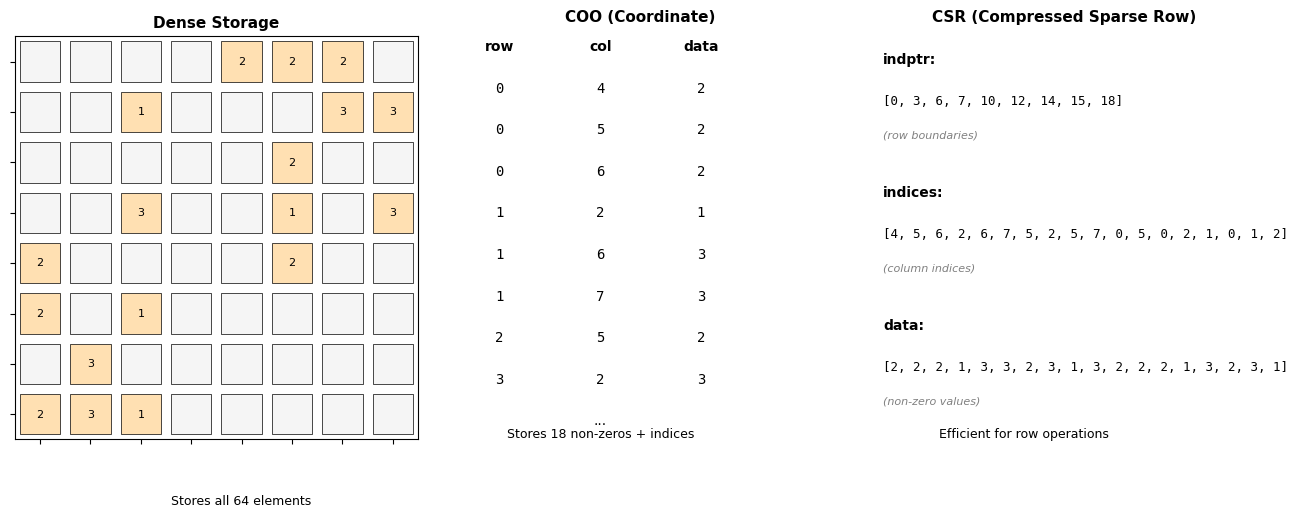
Format Selection
- COO: Best for construction and adding entries
- CSR: Best for row slicing and matrix-vector products
- CSC: Best for column slicing and linear solvers
import scipy.sparse as sp import numpy as np # Create sparse matrix n = 1000 density = 0.01 A_dense = sp.rand(n, n, density=density, format='dense') A_dense = np.array(A_dense) # Convert to different formats A_coo = sp.coo_matrix(A_dense) A_csr = sp.csr_matrix(A_dense) A_csc = sp.csc_matrix(A_dense) # Memory usage import sys dense_size = sys.getsizeof(A_dense) / 1024**2 coo_size = (A_coo.data.nbytes + A_coo.row.nbytes + A_coo.col.nbytes) / 1024**2 csr_size = (A_csr.data.nbytes + A_csr.indices.nbytes + A_csr.indptr.nbytes) / 1024**2 print(f"Matrix {n}×{n}, density {density:.1%}") print(f"Dense: {dense_size:.2f} MB") print(f"COO: {coo_size:.2f} MB ({dense_size/coo_size:.1f}× smaller)") print(f"CSR: {csr_size:.2f} MB ({dense_size/csr_size:.1f}× smaller)") # Operation performance v = np.random.randn(n) import timeit t_dense = timeit.timeit(lambda: A_dense @ v, number=100) t_csr = timeit.timeit(lambda: A_csr @ v, number=100) print(f"\nMatrix-vector multiply (100 iterations):") print(f"Dense: {t_dense*1000:.1f}ms") print(f"CSR: {t_csr*1000:.1f}ms ({t_dense/t_csr:.1f}× faster)") # Format conversion cost t_to_csr = timeit.timeit( lambda: sp.csr_matrix(A_dense), number=10 ) print(f"\nConversion to CSR: {t_to_csr*100:.1f}ms")
Matrix 1000×1000, density 1.0%
Dense: 7.63 MB
COO: 0.15 MB (50.0× smaller)
CSR: 0.12 MB (64.5× smaller)
Matrix-vector multiply (100 iterations):
Dense: 1.7ms
CSR: 0.5ms (3.1× faster)
Conversion to CSR: 2.4ms
Storage Format Trade-offs:
COO (Coordinate):
- Three arrays: (row, col, data)
- No sorting required
- Allows duplicates (summed on conversion)
- Inefficient for arithmetic
CSR/CSC (Compressed Sparse Row/Column):
- Row-wise: (indptr, indices, data)
- Efficient row/column access
- Fast matrix-vector products
- Standard solver format
Performance Implications:
- Dense wins below ~10% density
- Format conversion has significant cost
- Row vs column access patterns matter
- In-place operations often impossible
Matplotlib Architecture: Object Hierarchy
Matplotlib uses a hierarchical object model that separates concerns across multiple abstraction levels.
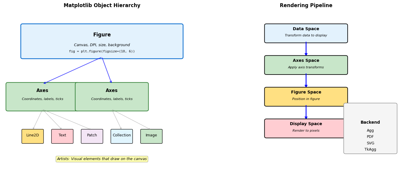
import matplotlib.pyplot as plt import matplotlib as mpl # Examine object hierarchy fig = plt.figure(figsize=(8, 4)) ax1 = fig.add_subplot(121) ax2 = fig.add_subplot(122) # Plot creates multiple artists line, = ax1.plot([1, 2, 3], [1, 4, 2], 'b-') scatter = ax2.scatter([1, 2, 3], [2, 3, 1]) # Object relationships print("Figure attributes:") print(f" Number of axes: {len(fig.axes)}") print(f" DPI: {fig.dpi}") print(f" Size: {fig.get_size_inches()} inches") print("\nAxes ax1 contents:") print(f" Lines: {len(ax1.lines)}") print(f" Patches: {len(ax1.patches)}") print(f" Texts: {len(ax1.texts)}") print(f" Artists: {len(ax1.get_children())}") # Access artist properties print(f"\nLine2D properties:") print(f" Data: x={line.get_xdata()}, y={line.get_ydata()}") print(f" Color: {line.get_color()}") print(f" Linewidth: {line.get_linewidth()}") print(f" Marker: '{line.get_marker()}'") # Transform pipeline data_point = (2, 4) display_point = ax1.transData.transform(data_point) figure_point = fig.transFigure.inverted().transform(display_point) print(f"\nTransform pipeline for {data_point}:") print(f" Data space: {data_point}") print(f" Display space: {display_point}") print(f" Figure space: {figure_point}") plt.close() # Clean up
Figure attributes:
Number of axes: 2
DPI: 100.0
Size: [8. 4.] inches
Axes ax1 contents:
Lines: 1
Patches: 0
Texts: 0
Artists: 11
Line2D properties:
Data: x=[1 2 3], y=[1 4 2]
Color: b
Linewidth: 2.0
Marker: 'None'
Transform pipeline for (2, 4):
Data space: (2, 4)
Display space: [ 663.63636364 1276. ]
Figure space: [0.82954545 3.19 ]
Architecture Components:
-
Figure: Top-level container
- Manages canvas and renderer
- Controls output size and DPI
- Contains one or more Axes
-
Axes: Plotting area with coordinates
- Data limits and scaling
- Tick locators and formatters
- Contains Artists
-
Artists: Everything visible
- Primitives: Line2D, Rectangle, Text
- Collections: LineCollection, PathCollection
- Containers: Axis, Legend
-
Transforms: Coordinate mappings
- Data → Axes → Figure → Display
- Enables zoom, pan, aspect ratio
-
Backend: Rendering engine
- Interactive: Qt5Agg, TkAgg
- Hardcopy: Agg, PDF, SVG
Plot Types for Scientific Data
Different visualizations optimize for different data characteristics and analysis goals.
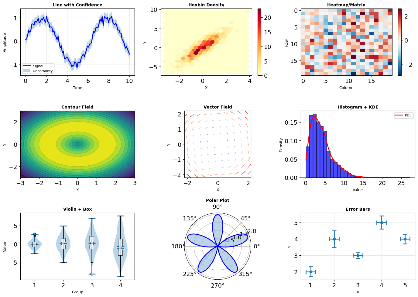
import matplotlib.pyplot as plt import numpy as np # Performance comparison for different plot types data_sizes = [100, 1000, 10000, 100000] plot_types = { 'line': lambda ax, n: ax.plot(np.arange(n), np.random.randn(n)), 'scatter': lambda ax, n: ax.scatter(np.arange(n), np.random.randn(n)), 'hist': lambda ax, n: ax.hist(np.random.randn(n), bins=50), 'imshow': lambda ax, n: ax.imshow(np.random.randn(int(np.sqrt(n)), int(np.sqrt(n)))), } import time print("Rendering time (ms) for different plot types:") print(f"{'Size':<10} {'Line':<10} {'Scatter':<10} {'Hist':<10} {'Imshow':<10}") print("-" * 50) for size in data_sizes: times = {} for plot_type, plot_func in plot_types.items(): fig, ax = plt.subplots() start = time.perf_counter() plot_func(ax, size) fig.canvas.draw() elapsed = (time.perf_counter() - start) * 1000 times[plot_type] = elapsed plt.close(fig) print(f"{size:<10} {times['line']:<10.1f} {times['scatter']:<10.1f} " f"{times['hist']:<10.1f} {times['imshow']:<10.1f}") # Memory usage analysis import sys fig, ax = plt.subplots() line, = ax.plot(np.arange(10000), np.random.randn(10000)) scatter = ax.scatter(np.arange(1000), np.random.randn(1000)) print(f"\nMemory usage:") print(f" Line (10k points): ~{sys.getsizeof(line.get_xydata()) / 1024:.1f} KB") print(f" Scatter (1k points): ~{sys.getsizeof(scatter.get_offsets()) / 1024:.1f} KB") plt.close()
Rendering time (ms) for different plot types:
Size Line Scatter Hist Imshow
--------------------------------------------------
100 8.4 7.7 15.8 10.5
1000 13.3 8.9 16.5 12.5
10000 58.5 12.7 15.8 10.9
100000 277.2 39.8 16.7 18.8
Memory usage:
Line (10k points): ~156.4 KB
Scatter (1k points): ~0.2 KB
Plot Selection Criteria:
Continuous Data:
- Line: Time series, functions
- Fill: Confidence intervals, ranges
- Contour: 2D scalar fields
Discrete Points:
- Scatter: Correlations, outliers
- Hexbin: Large datasets (>10k points)
- Histogram: Distributions
Statistical:
- Box: Quartiles and outliers
- Violin: Distribution shape
- Error bars: Measurement uncertainty
Performance Tips:
- Use
plot()overscatter()for large datasets - Rasterize dense plots:
rasterized=True - Downsample data before plotting
- Use blitting for animations
Subplot Layouts and Composition
Complex figures require careful layout management for effective visualization.
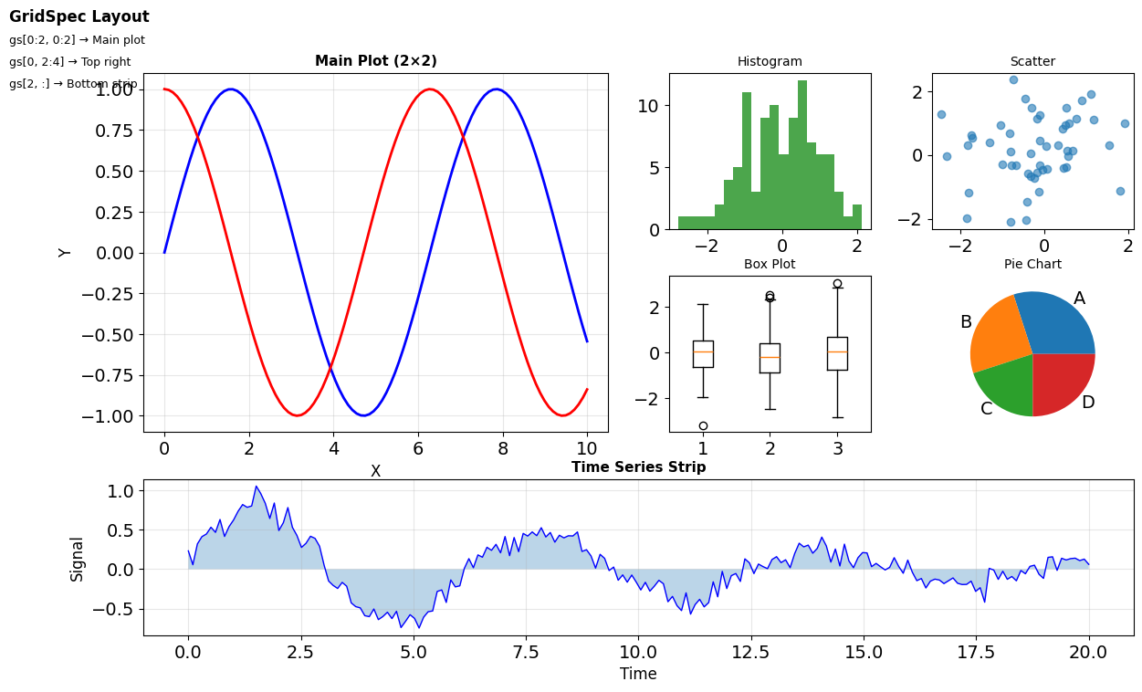
import matplotlib.pyplot as plt import matplotlib.gridspec as gridspec import numpy as np # Method 1: Simple grid fig1, axes = plt.subplots(2, 3, figsize=(9, 6)) print(f"Simple grid: {axes.shape} axes") # Method 2: GridSpec for complex layouts fig2 = plt.figure(figsize=(10, 6)) gs = gridspec.GridSpec(3, 3, figure=fig2, width_ratios=[1, 2, 1], height_ratios=[1, 2, 1], hspace=0.3, wspace=0.3) # Create axes with different spans ax1 = fig2.add_subplot(gs[0, :]) # Top row, all columns ax2 = fig2.add_subplot(gs[1:, 0]) # Rows 1-2, first column ax3 = fig2.add_subplot(gs[1:, 1:]) # Rows 1-2, columns 1-2 print(f"\nGridSpec axes positions:") print(f" ax1: {ax1.get_position()}") print(f" ax2: {ax2.get_position()}") print(f" ax3: {ax3.get_position()}") # Method 3: Nested layouts fig3 = plt.figure(figsize=(10, 6)) outer_grid = gridspec.GridSpec(2, 2, figure=fig3) # Nested grid in first cell inner_grid = gridspec.GridSpecFromSubplotSpec( 2, 2, subplot_spec=outer_grid[0, 0] ) # Create nested axes for i in range(2): for j in range(2): ax = fig3.add_subplot(inner_grid[i, j]) ax.text(0.5, 0.5, f'({i},{j})', ha='center') # Regular axes in other cells ax_right = fig3.add_subplot(outer_grid[0, 1]) ax_bottom = fig3.add_subplot(outer_grid[1, :]) plt.close('all') # Clean up # Constrained layout for automatic spacing fig4, axes = plt.subplots(2, 2, figsize=(8, 6), constrained_layout=True) for ax in axes.flat: ax.plot(np.random.randn(100)) ax.set_title('Auto-spaced') print("\nConstrained layout automatically adjusts spacing") plt.close('all')
Simple grid: (2, 3) axes
GridSpec axes positions:
ax1: Bbox(x0=0.125, y0=0.7195833333333334, x1=0.9000000000000001, y1=0.88)
ax2: Bbox(x0=0.125, y0=0.10999999999999999, x1=0.28645833333333337, y1=0.6554166666666668)
ax3: Bbox(x0=0.3510416666666667, y0=0.10999999999999999, x1=0.9000000000000001, y1=0.6554166666666668)
Constrained layout automatically adjusts spacing
# Shared axes for comparison fig, axes = plt.subplots(3, 1, figsize=(8, 6), sharex=True) x = np.linspace(0, 10, 100) data = [np.sin(x), np.cos(x), np.sin(x) * np.cos(x)] labels = ['sin(x)', 'cos(x)', 'sin(x)cos(x)'] for ax, y, label in zip(axes, data, labels): ax.plot(x, y, linewidth=2) ax.set_ylabel(label) ax.grid(True, alpha=0.3) # Only bottom axis shows x-label if ax == axes[-1]: ax.set_xlabel('X') axes[0].set_title('Shared X-axis', fontweight='bold') # Measure rendering overhead import time layout_times = {} # Simple layout start = time.perf_counter() fig, axes = plt.subplots(3, 3) fig.canvas.draw() layout_times['simple'] = time.perf_counter() - start # Complex GridSpec start = time.perf_counter() fig = plt.figure() gs = gridspec.GridSpec(5, 5) for i in range(5): for j in range(5): ax = fig.add_subplot(gs[i, j]) fig.canvas.draw() layout_times['complex'] = time.perf_counter() - start print("\nLayout creation overhead:") for layout, t in layout_times.items(): print(f" {layout}: {t*1000:.1f}ms") plt.close('all')
Layout creation overhead:
simple: 58.6ms
complex: 109.2ms
3D Visualization
Three-dimensional plots require special consideration for perspective and interaction.
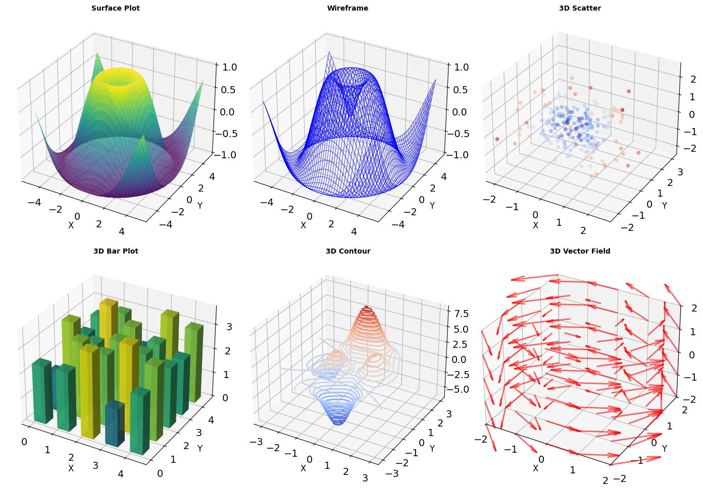
from mpl_toolkits.mplot3d import Axes3D import numpy as np import time # Performance analysis for 3D plots fig = plt.figure(figsize=(10, 5)) # Compare 2D vs 3D rendering grid_sizes = [10, 20, 30, 40, 50] times_2d = [] times_3d = [] for size in grid_sizes: X = np.linspace(-5, 5, size) Y = np.linspace(-5, 5, size) X, Y = np.meshgrid(X, Y) Z = np.sin(np.sqrt(X**2 + Y**2)) # 2D heatmap fig2d, ax2d = plt.subplots() start = time.perf_counter() ax2d.imshow(Z) fig2d.canvas.draw() times_2d.append(time.perf_counter() - start) plt.close(fig2d) # 3D surface fig3d = plt.figure() ax3d = fig3d.add_subplot(111, projection='3d') start = time.perf_counter() ax3d.plot_surface(X, Y, Z) fig3d.canvas.draw() times_3d.append(time.perf_counter() - start) plt.close(fig3d) print("Rendering time comparison (ms):") print(f"{'Grid':<10} {'2D Heatmap':<15} {'3D Surface':<15} {'Ratio':<10}") print("-" * 50) for i, size in enumerate(grid_sizes): ratio = times_3d[i] / times_2d[i] print(f"{size}×{size:<6} {times_2d[i]*1000:<15.1f} " f"{times_3d[i]*1000:<15.1f} {ratio:<10.1f}x") # View angle impact fig = plt.figure() ax = fig.add_subplot(111, projection='3d') # Create surface X = np.linspace(-5, 5, 30) Y = np.linspace(-5, 5, 30) X, Y = np.meshgrid(X, Y) Z = np.sin(np.sqrt(X**2 + Y**2)) ax.plot_surface(X, Y, Z, cmap='viridis') # Get view angles elev = ax.elev azim = ax.azim print(f"\nDefault view angles:") print(f" Elevation: {elev}°") print(f" Azimuth: {azim}°") # Programmatic rotation ax.view_init(elev=30, azim=45) print(f"Modified view: elev=30°, azim=45°") plt.close()
Rendering time comparison (ms):
Grid 2D Heatmap 3D Surface Ratio
--------------------------------------------------
10×10 11.5 14.1 1.2 x
20×20 14.4 18.9 1.3 x
30×30 11.8 27.3 2.3 x
40×40 15.0 38.4 2.6 x
50×50 11.3 53.3 4.7 x
Default view angles:
Elevation: 30°
Azimuth: -60°
Modified view: elev=30°, azim=45°
<Figure size 1000x500 with 0 Axes># 3D plotting optimizations import matplotlib.pyplot as plt from mpl_toolkits.mplot3d import Axes3D import numpy as np # Optimization strategies fig = plt.figure(figsize=(8, 4)) # Strategy 1: Reduce resolution ax1 = fig.add_subplot(121, projection='3d') X_low = np.linspace(-5, 5, 20) # Low resolution Y_low = np.linspace(-5, 5, 20) X_low, Y_low = np.meshgrid(X_low, Y_low) Z_low = np.sin(np.sqrt(X_low**2 + Y_low**2)) ax1.plot_surface(X_low, Y_low, Z_low, cmap='viridis', alpha=0.8) ax1.set_title('Low Resolution (Fast)') # Strategy 2: Use simpler representations ax2 = fig.add_subplot(122, projection='3d') ax2.plot_wireframe(X_low, Y_low, Z_low, color='blue', linewidth=0.5, rstride=2, cstride=2) # Skip points ax2.set_title('Wireframe (Faster)') # Memory usage import sys surf_artist = ax1.collections[0] wire_artist = ax2.collections[0] print("\nMemory comparison:") print(f" Surface plot: ~{len(surf_artist._facecolors)*4/1024:.1f} KB") print(f" Wireframe: ~{len(wire_artist._segments3d)*24/1024:.1f} KB") # Z-order sorting overhead n_triangles = X_low.size * 2 # Approximate print(f"\nZ-buffer sorting:") print(f" Triangles to sort: ~{n_triangles}") print(f" Complexity: O(n log n) = O({n_triangles} log {n_triangles})") plt.tight_layout() plt.close() # Interactive considerations print("\n3D interaction overhead:") print(" Mouse rotation: Recomputes projections") print(" Zoom: Recalculates clipping") print(" Pan: Updates transform matrices")
Memory comparison:
Surface plot: ~0.0 KB
Wireframe: ~0.5 KB
Z-buffer sorting:
Triangles to sort: ~800
Complexity: O(n log n) = O(800 log 800)
3D interaction overhead:
Mouse rotation: Recomputes projections
Zoom: Recalculates clipping
Pan: Updates transform matrices
Animations for Time Series
Animations visualize temporal evolution but require careful performance optimization.
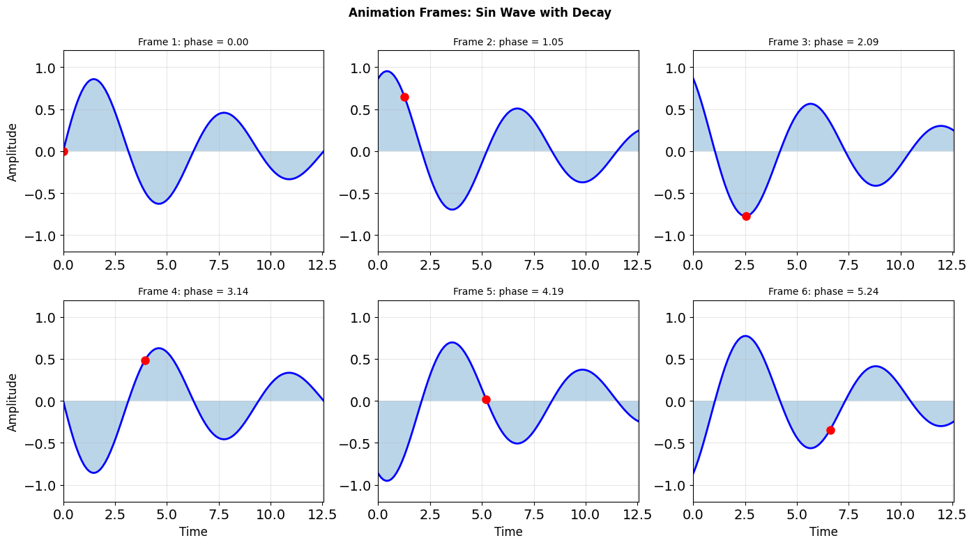
import matplotlib.pyplot as plt import matplotlib.animation as animation import numpy as np # Basic animation structure fig, (ax1, ax2) = plt.subplots(2, 1, figsize=(8, 6)) # Data setup x = np.linspace(0, 2*np.pi, 100) line1, = ax1.plot([], [], 'b-', linewidth=2) line2, = ax2.plot([], [], 'r-', linewidth=2) ax1.set_xlim(0, 2*np.pi) ax1.set_ylim(-1.5, 1.5) ax1.set_title('Animation with Blitting') ax1.grid(True, alpha=0.3) ax2.set_xlim(0, 2*np.pi) ax2.set_ylim(-1.5, 1.5) ax2.set_title('Accumulated History') ax2.grid(True, alpha=0.3) # Animation state history = [] def init(): """Initialize animation.""" line1.set_data([], []) line2.set_data([], []) return line1, line2 def animate(frame): """Animation function called for each frame.""" # Update data y1 = np.sin(x + frame * 0.1) line1.set_data(x, y1) # Accumulate history if len(history) > 50: history.pop(0) history.append(np.sin(2*np.pi * frame / 50)) # Plot history if history: line2.set_data(np.linspace(0, 2*np.pi, len(history)), history) return line1, line2 # Performance comparison import time # Without blitting start = time.perf_counter() for i in range(50): animate(i) fig.canvas.draw() no_blit_time = time.perf_counter() - start print(f"Animation performance (50 frames):") print(f" Without blitting: {no_blit_time*1000:.1f}ms") print(f" FPS: {50/no_blit_time:.1f}") # Memory management print(f"\nMemory considerations:") print(f" Line data: {x.nbytes + x.nbytes} bytes per frame") print(f" History buffer: {len(history) * 8} bytes") print(f" Canvas cache: ~{fig.canvas.get_width_height()[0] * fig.canvas.get_width_height()[1] * 4} bytes") plt.close() # Optimization techniques print("\nOptimization strategies:") print(" 1. Use blitting: ~5-10x speedup") print(" 2. Update only changed artists") print(" 3. Reduce figure DPI for preview") print(" 4. Cache static elements") print(" 5. Use collections for many objects")
Animation performance (50 frames):
Without blitting: 531.2ms
FPS: 94.1
Memory considerations:
Line data: 1600 bytes per frame
History buffer: 400 bytes
Canvas cache: ~1920000 bytes
Optimization strategies:
1. Use blitting: ~5-10x speedup
2. Update only changed artists
3. Reduce figure DPI for preview
4. Cache static elements
5. Use collections for many objects
Animation structure:
# Create figure and line artist fig, ax = plt.subplots() line, = ax.plot([], []) def init(): """Set up blank frame.""" line.set_data([], []) return line, def animate(frame): """Update for each frame.""" y = np.sin(x + frame * 0.1) line.set_data(x, y) return line, # Create animation anim = FuncAnimation(fig, animate, init_func=init, frames=100, interval=50, blit=True) # Save to file anim.save('animation.mp4', writer='ffmpeg', fps=30)
Blitting caches the static background and redraws only the changed artists — typically 5-10x faster than full redraws.
blit=True requires:
init()andanimate()return iterables of updated artists- Artists must be on the same axes
- Background must not change between frames
Saving animations:
- MP4:
writer='ffmpeg'(requires ffmpeg installed) - GIF:
writer='pillow' - HTML5:
anim.to_jshtml()for notebooks
Performance Optimization for Large Datasets
Visualizing large datasets requires strategic optimization to maintain interactivity.
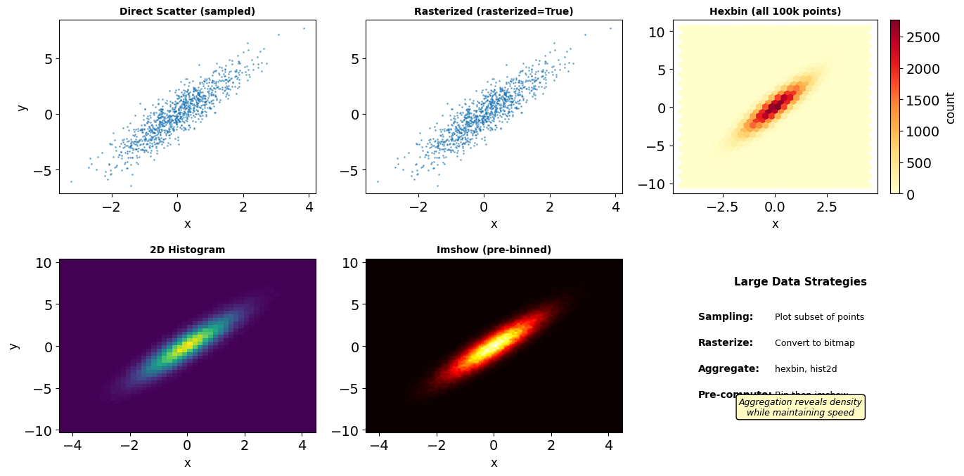
import matplotlib.pyplot as plt import numpy as np import time # Generate large dataset n_points = 50000 x = np.random.randn(n_points) y = 2*x + np.random.randn(n_points) # Benchmark different approaches results = {} # 1. Direct scatter (limited to 5k for speed) fig, ax = plt.subplots() start = time.perf_counter() ax.scatter(x[:5000], y[:5000], alpha=0.5, s=1) fig.canvas.draw() results['scatter_5k'] = time.perf_counter() - start plt.close() # 2. Plot instead of scatter fig, ax = plt.subplots() start = time.perf_counter() ax.plot(x, y, 'o', markersize=1, alpha=0.5) fig.canvas.draw() results['plot_50k'] = time.perf_counter() - start plt.close() # 3. Hexbin fig, ax = plt.subplots() start = time.perf_counter() ax.hexbin(x, y, gridsize=30) fig.canvas.draw() results['hexbin_50k'] = time.perf_counter() - start plt.close() # 4. 2D histogram fig, ax = plt.subplots() start = time.perf_counter() ax.hist2d(x, y, bins=50) fig.canvas.draw() results['hist2d_50k'] = time.perf_counter() - start plt.close() print("Rendering performance:") for method, time_val in results.items(): print(f" {method:15s}: {time_val*1000:6.1f}ms") # Memory usage estimation import sys # Scatter artist memory fig, ax = plt.subplots() scatter = ax.scatter(x[:1000], y[:1000]) scatter_memory = (sys.getsizeof(scatter.get_offsets()) + sys.getsizeof(scatter.get_facecolors())) # Line artist memory line, = ax.plot(x[:1000], y[:1000], 'o') line_memory = sys.getsizeof(line.get_xydata()) print(f"\nMemory usage (1000 points):") print(f" Scatter: ~{scatter_memory/1024:.1f} KB") print(f" Line: ~{line_memory/1024:.1f} KB") print(f" Ratio: {scatter_memory/line_memory:.1f}x") plt.close('all')
Rendering performance:
scatter_5k : 10.8ms
plot_50k : 12.5ms
hexbin_50k : 16.5ms
hist2d_50k : 12.7ms
Memory usage (1000 points):
Scatter: ~0.3 KB
Line: ~15.8 KB
Ratio: 0.0x
# Optimization strategies class OptimizedPlotter: """Strategies for large dataset visualization.""" @staticmethod def downsample(x, y, max_points=1000): """Randomly sample if too many points.""" n = len(x) if n <= max_points: return x, y idx = np.random.choice(n, max_points, replace=False) return x[idx], y[idx] @staticmethod def use_rasterization(ax, x, y): """Rasterize dense plots.""" ax.scatter(x, y, alpha=0.5, s=1, rasterized=True) # Rasterized elements become bitmaps # Faster zooming/panning @staticmethod def aggregate_data(x, y, bins=50): """Convert to density representation.""" H, xedges, yedges = np.histogram2d(x, y, bins=bins) return H, xedges, yedges @staticmethod def progressive_rendering(x, y, ax): """Render in stages for responsiveness.""" # Quick preview x_preview, y_preview = OptimizedPlotter.downsample( x, y, max_points=100 ) line = ax.plot(x_preview, y_preview, 'o', markersize=2, alpha=0.3)[0] ax.figure.canvas.draw() # Full render line.set_data(x, y) ax.figure.canvas.draw() # Level-of-detail (LOD) system class LODPlot: """Adaptive detail based on zoom level.""" def __init__(self, x, y): self.x_full = x self.y_full = y self.create_levels() def create_levels(self): """Create multiple resolution levels.""" self.levels = {} n = len(self.x_full) # Full resolution self.levels[0] = (self.x_full, self.y_full) # Reduced resolutions for level in [1, 2, 3]: step = 2 ** level self.levels[level] = ( self.x_full[::step], self.y_full[::step] ) def get_data(self, zoom_level): """Return appropriate resolution.""" if zoom_level > 10: return self.levels[0] # Full elif zoom_level > 5: return self.levels[1] # Half elif zoom_level > 2: return self.levels[2] # Quarter else: return self.levels[3] # Eighth # Test LOD system lod = LODPlot(x, y) print("\nLOD system points at each level:") for level in range(4): x_level, y_level = lod.levels[level] print(f" Level {level}: {len(x_level)} points") # Chunked rendering for streaming def chunked_plot(x, y, ax, chunk_size=5000): """Plot data in chunks to maintain responsiveness.""" n_chunks = len(x) // chunk_size + 1 for i in range(n_chunks): start = i * chunk_size end = min((i + 1) * chunk_size, len(x)) ax.plot(x[start:end], y[start:end], 'o', markersize=1, alpha=0.5) # Allow GUI to update if i % 5 == 0: ax.figure.canvas.draw() plt.pause(0.001) print("\nOptimization impact:") print(" Rasterization: 2-5x faster interaction") print(" Aggregation: 10-100x data reduction") print(" LOD: Adaptive performance")
LOD system points at each level:
Level 0: 50000 points
Level 1: 25000 points
Level 2: 12500 points
Level 3: 6250 points
Optimization impact:
Rasterization: 2-5x faster interaction
Aggregation: 10-100x data reduction
LOD: Adaptive performance
Backend Selection and Output Formats
Different backends optimize for different use cases: interactivity vs. publication quality.
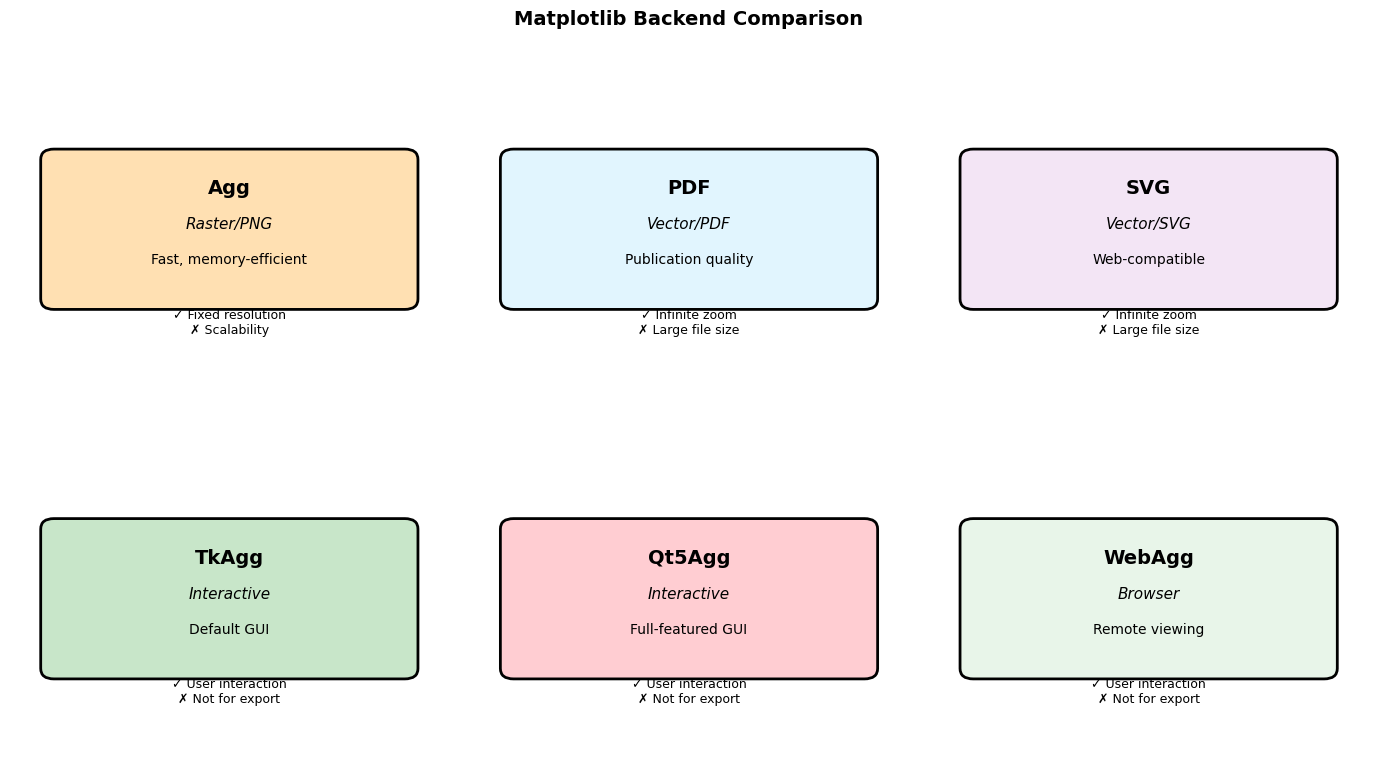
import matplotlib import matplotlib.pyplot as plt import numpy as np import os # Check available backends print("Available backends:") for backend in matplotlib.rcsetup.all_backends: print(f" {backend}") print(f"\nCurrent backend: {matplotlib.get_backend()}") # Create test figure fig, ax = plt.subplots(figsize=(6, 4)) x = np.linspace(0, 10, 1000) ax.plot(x, np.sin(x), 'b-', linewidth=2) ax.fill_between(x, 0, np.sin(x), alpha=0.3) ax.set_title('Test Figure') ax.grid(True, alpha=0.3) # Save in different formats formats = { 'png': {'dpi': 100, 'bbox_inches': 'tight'}, 'pdf': {'bbox_inches': 'tight'}, 'svg': {'bbox_inches': 'tight'}, 'eps': {'bbox_inches': 'tight'}, } file_sizes = {} import time for fmt, kwargs in formats.items(): filename = f'test_figure.{fmt}' start = time.perf_counter() fig.savefig(filename, format=fmt, **kwargs) save_time = time.perf_counter() - start # Check file size if os.path.exists(filename): size = os.path.getsize(filename) / 1024 # KB file_sizes[fmt] = (size, save_time) os.remove(filename) # Clean up print("\nOutput format comparison:") print(f"{'Format':<10} {'Size (KB)':<12} {'Time (ms)':<10}") print("-" * 35) for fmt, (size, save_time) in file_sizes.items(): print(f"{fmt:<10} {size:<12.1f} {save_time*1000:<10.1f}") plt.close() # DPI impact on file size dpis = [72, 100, 150, 200, 300] sizes = [] times = [] for dpi in dpis: start = time.perf_counter() fig.savefig('temp.png', dpi=dpi) times.append(time.perf_counter() - start) sizes.append(os.path.getsize('temp.png') / 1024) os.remove('temp.png') print("\nDPI impact (PNG):") print(f"{'DPI':<10} {'Size (KB)':<12} {'Time (ms)':<10}") print("-" * 35) for dpi, size, save_time in zip(dpis, sizes, times): print(f"{dpi:<10} {size:<12.1f} {save_time*1000:<10.1f}")
Available backends:
gtk3agg
gtk3cairo
gtk4agg
gtk4cairo
macosx
nbagg
notebook
qtagg
qtcairo
qt5agg
qt5cairo
tkagg
tkcairo
webagg
wx
wxagg
wxcairo
agg
cairo
pdf
pgf
ps
svg
template
Current backend: module://matplotlib_inline.backend_inline
Output format comparison:
Format Size (KB) Time (ms)
-----------------------------------
png 21.8 18.4
pdf 23.2 389.4
svg 68.8 20.8
eps 62.9 20.8
DPI impact (PNG):
DPI Size (KB) Time (ms)
-----------------------------------
72 14.6 7.3
100 22.2 8.6
150 34.2 11.6
200 49.0 16.1
300 77.6 28.5
# Backend-specific optimizations import matplotlib.pyplot as plt import numpy as np # Configure for publication def setup_publication(): """Configure matplotlib for publication.""" plt.rcParams.update({ 'font.size': 10, 'font.family': 'serif', 'text.usetex': False, # Set True for LaTeX 'axes.linewidth': 1.5, 'axes.labelsize': 11, 'axes.titlesize': 12, 'xtick.labelsize': 10, 'ytick.labelsize': 10, 'legend.fontsize': 10, 'figure.dpi': 100, 'savefig.dpi': 300, 'savefig.bbox': 'tight', 'savefig.pad_inches': 0.1, }) # Configure for presentation def setup_presentation(): """Configure matplotlib for slides.""" plt.rcParams.update({ 'font.size': 14, 'font.family': 'sans-serif', 'axes.linewidth': 2, 'axes.labelsize': 16, 'axes.titlesize': 18, 'lines.linewidth': 3, 'lines.markersize': 10, 'xtick.labelsize': 14, 'ytick.labelsize': 14, 'legend.fontsize': 14, 'figure.dpi': 100, 'savefig.dpi': 150, }) # Backend-specific features def interactive_features(): """Features only available in interactive backends.""" fig, ax = plt.subplots() ax.plot([1, 2, 3], [1, 4, 2]) # Only works with interactive backends if matplotlib.get_backend().endswith('Agg'): print("Non-interactive backend - no GUI features") else: # These would work in interactive mode print("Interactive features available:") print(" - fig.canvas.mpl_connect('button_press_event', callback)") print(" - plt.ginput(n=3) # Get n mouse clicks") print(" - plt.waitforbuttonpress()") plt.close() interactive_features() # Format selection guide print("\nFormat selection guide:") print(" PNG: Web, general use, fixed resolution") print(" PDF: LaTeX, publications, vector graphics") print(" SVG: Web animations, editing, vector") print(" EPS: Legacy publications, PostScript") # Memory vs quality tradeoff print("\nMemory/Quality tradeoffs:") print(" Rasterized=True: Reduces PDF size for dense plots") print(" DPI: Higher = better quality, larger files") print(" Compression: PNG supports lossless compression")
Interactive features available:
- fig.canvas.mpl_connect('button_press_event', callback)
- plt.ginput(n=3) # Get n mouse clicks
- plt.waitforbuttonpress()
Format selection guide:
PNG: Web, general use, fixed resolution
PDF: LaTeX, publications, vector graphics
SVG: Web animations, editing, vector
EPS: Legacy publications, PostScript
Memory/Quality tradeoffs:
Rasterized=True: Reduces PDF size for dense plots
DPI: Higher = better quality, larger files
Compression: PNG supports lossless compression