Generalization is the Goal of Machine Learning
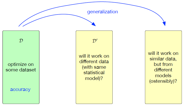
- Do not care about performance on the dataset we have
- Do care about performance on similar data that has no labels
- Accuracy/Generalization trade-off (bias-variance trade):
- Optimizing accuracy to the extreme reduces capability to generalize
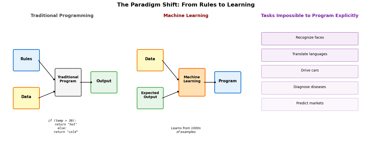
Machine Learning Inverts Traditional Programming
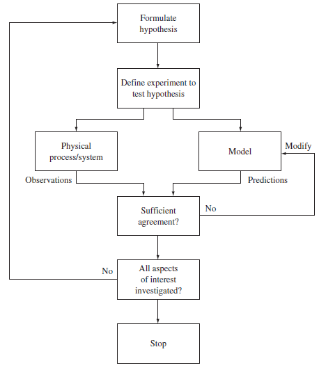
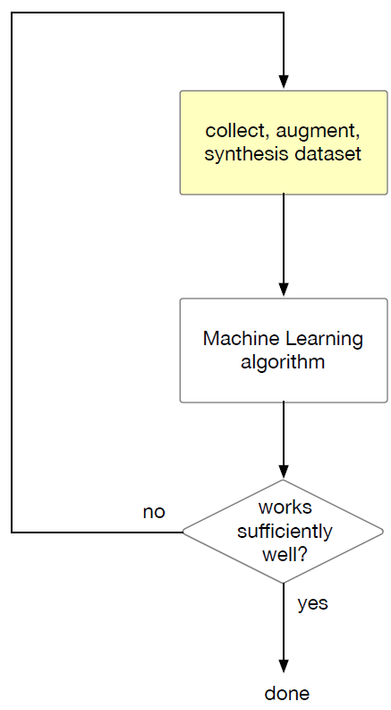
Theory-Driven vs Data-Driven Approaches
Classical: Theory-Driven
Modern: Data-Driven
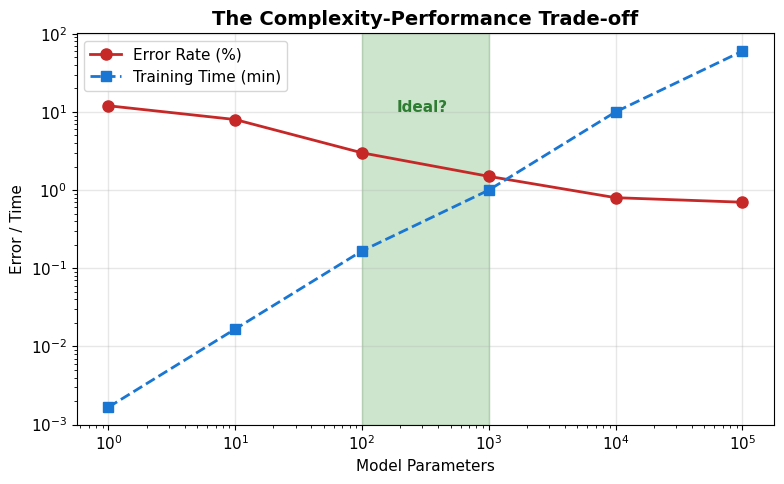
Model Complexity: When to Stop Adding Parameters
George Box (1976)
“All models are wrong, but some are useful”
“Since all models are wrong the scientist cannot obtain a ‘correct’ one by excessive elaboration”
Box’s warning: More parameters ≠ better science
MNIST Classification: Accuracy vs Complexity
- Nearest neighbor: 3% error, \(\mathcal{O}(n)\) inference
- Linear classifier: 8% error, \(\mathcal{O}(d)\) inference
- 2-layer network: 2% error, 50K parameters
- ConvNet (LeNet-5): 0.8% error, 60K parameters
- ResNet-50: 0.2% error, 25M parameters
Question: Is 0.2% → 0.1% worth 25M parameters?
Worrying Selectively
It is inappropriate to be concerned about mice when there are tigers abroad
- Start simple
- Add complexity purposefully
- Validate empirically
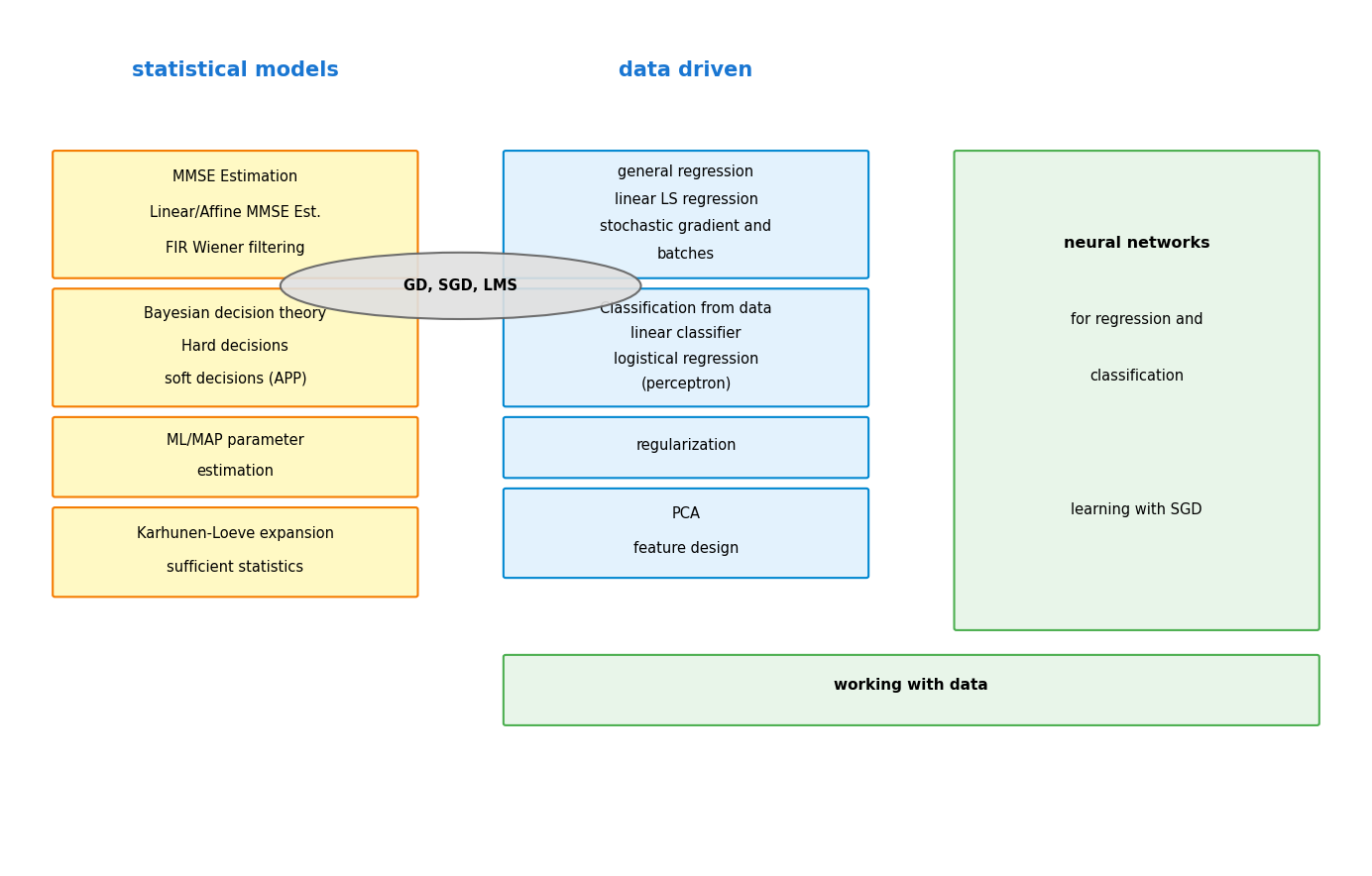
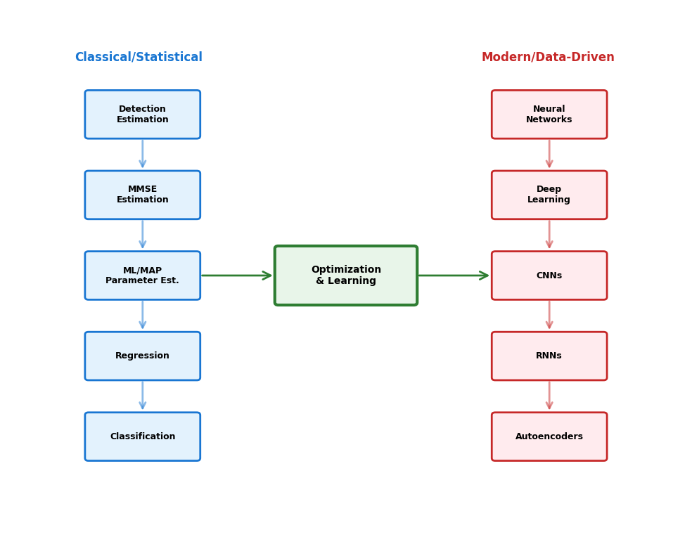
Course Structure: Statistical Foundations to Neural Networks
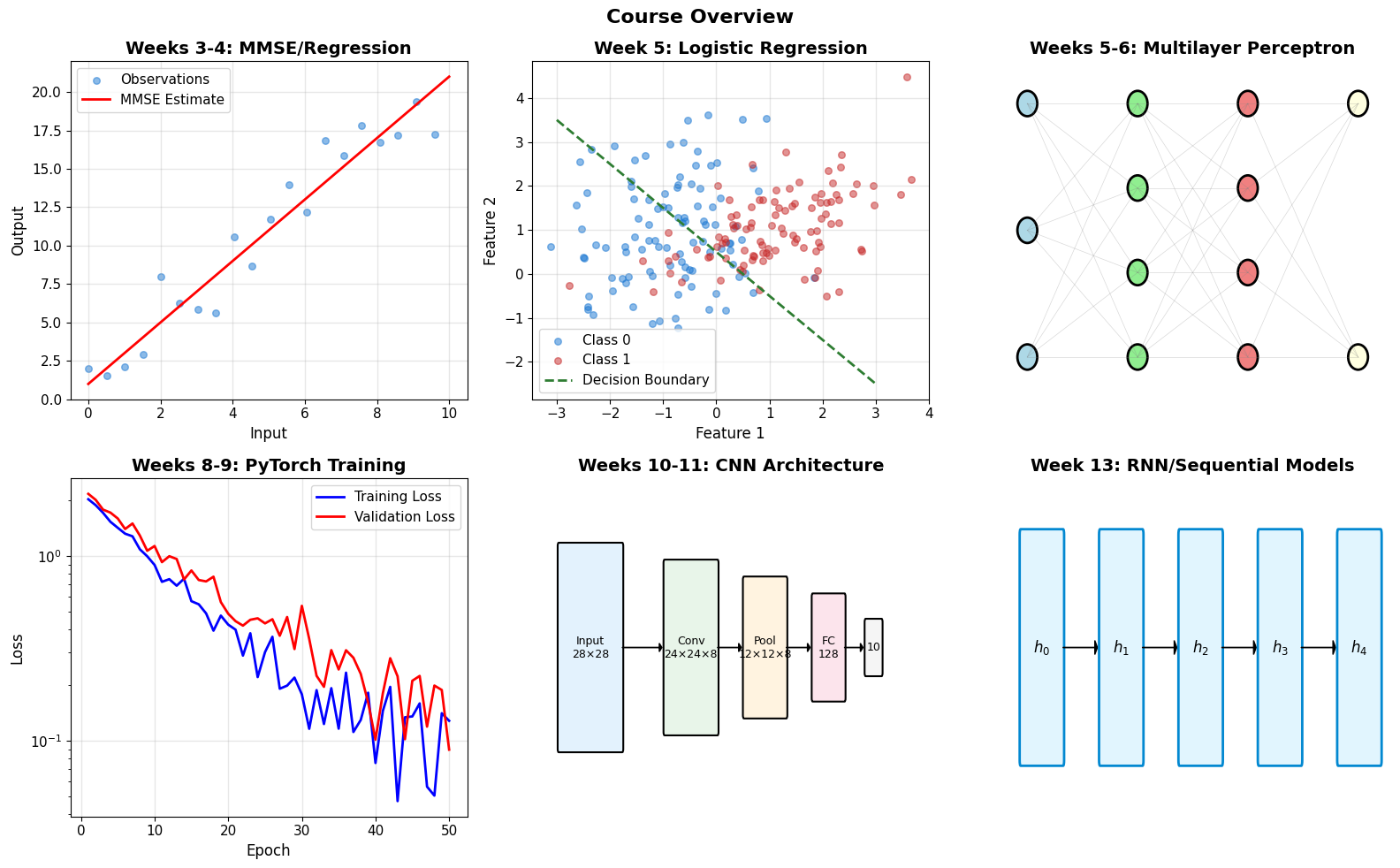
Semester Progression: MMSE to Convolutional Networks
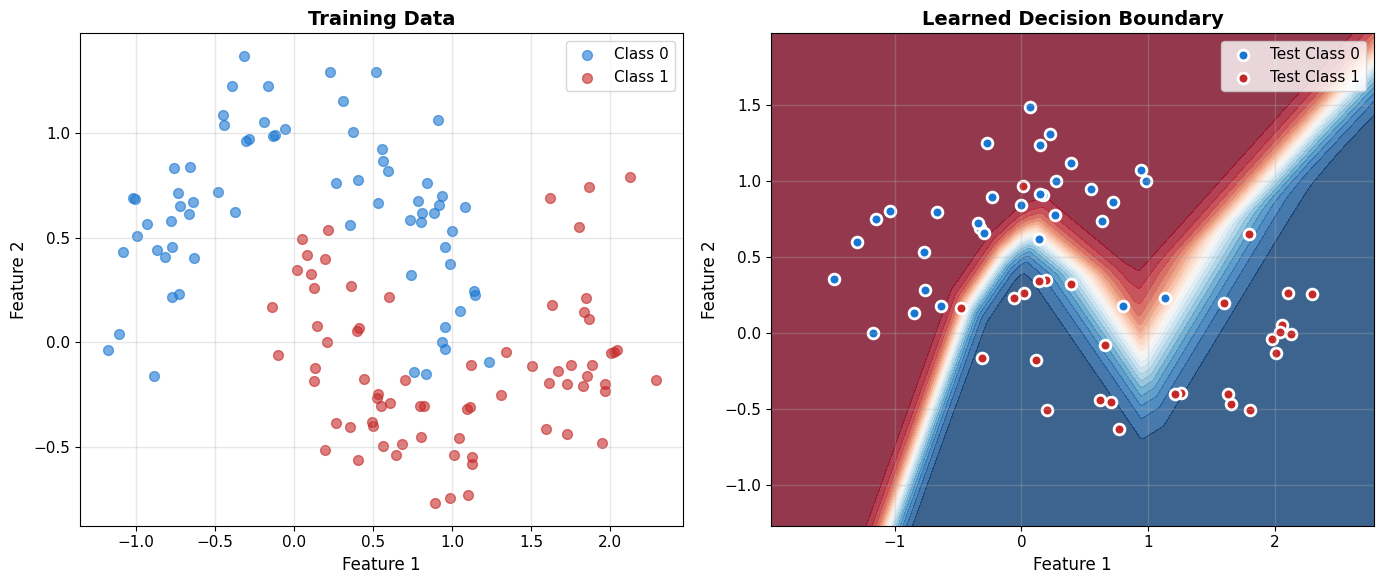
Linear Models Fail on Nonlinear Boundaries
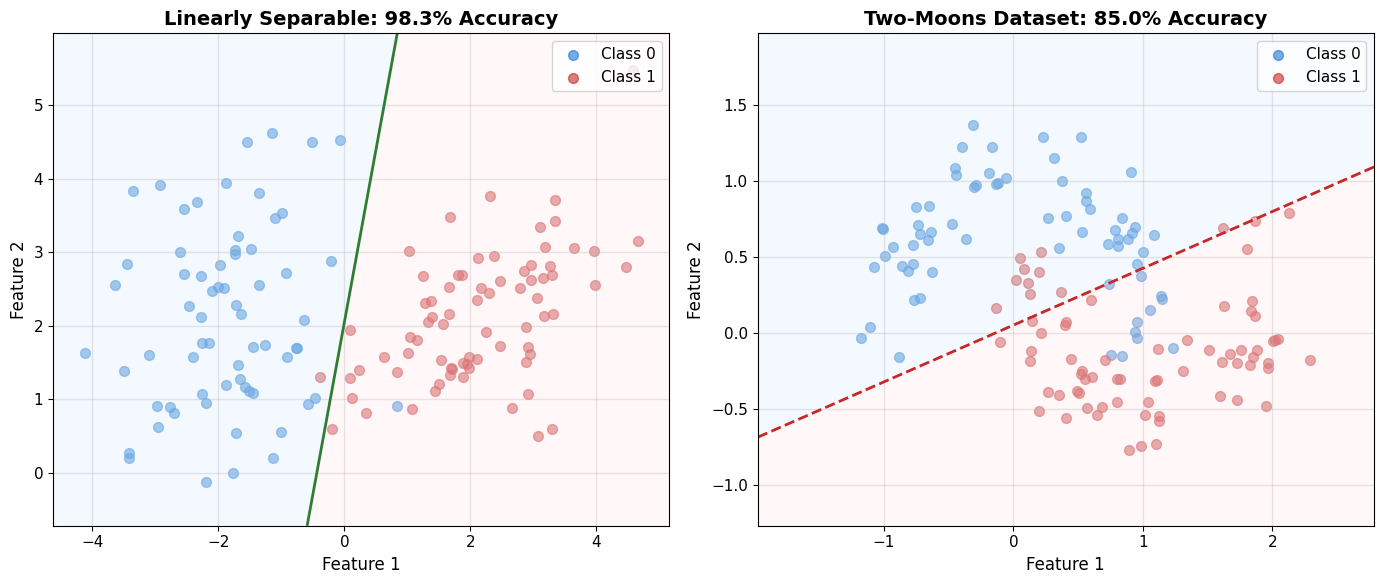
Two-Moons Dataset
Tests whether a model can learn curved decision boundaries. Two interleaving half-circles that cannot be separated by any straight line.
Neural Networks Learn Nonlinear Decision Boundaries
Code
import numpy as np
from sklearn.neural_network import MLPClassifier
from sklearn.datasets import make_moons
from sklearn.model_selection import train_test_split

X, y = make_moons(n_samples=200, noise=0.2, random_state=42)
X_train, X_test, y_train, y_test = train_test_split(
    X, y, test_size=0.3, random_state=42
)

mlp = MLPClassifier(
    hidden_layer_sizes=(10, 10),
    max_iter=1000,
    random_state=42
)
mlp.fit(X_train, y_train)

print(f"Training accuracy: {mlp.score(X_train, y_train):.3f}")
print(f"Test accuracy: {mlp.score(X_test, y_test):.3f}")
Training accuracy: 0.979
Test accuracy: 0.950
Minimize Expected Risk Using Only Finite Samples
Given
- Training data: \(\mathcal{D} = \{(\mathbf{x}_i, y_i)\}_{i=1}^N\)
- Hypothesis class: \(\mathcal{H}\)
- Loss function: \(\mathcal{L}\)
Goal
Find \(h^* \in \mathcal{H}\) that minimizes:
\[\mathbb{E}_{(\mathbf{x},y) \sim P}[\mathcal{L}(h(\mathbf{x}), y)]\]
But we only have access to:
\[\frac{1}{N}\sum_{i=1}^N \mathcal{L}(h(\mathbf{x}_i), y_i)\]
Generalization Gap
Minimize error on unseen data using only observed samples
This gap defines machine learning
Example Task: “2s” Detector
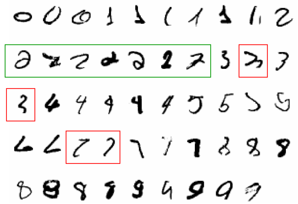
MNIST: Input and Output Representations
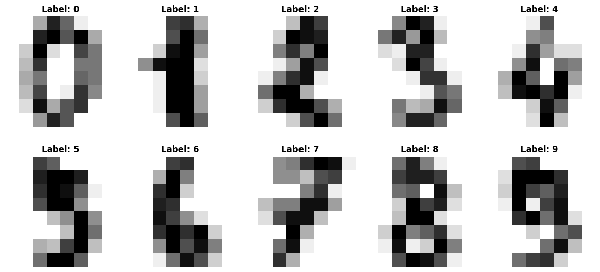
Input Space
- Raw pixels: \(\mathbf{x} \in \{0,255\}^{784}\)
- Normalized: \(\mathbf{x} \in [0,1]^{784}\)
- Binary: \(\mathbf{x} \in \{0,1\}^{784}\)
Output Space
- Classification: \(y \in \{0,1,...,9\}\)
- One-hot: \(\mathbf{y} \in \{0,1\}^{10}\)
- Probability: \(\mathbf{y} \in [0,1]^{10}\)
Same Data, Multiple Representations
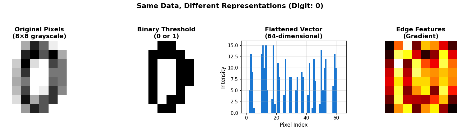
Representation Determines Learnability
The choice of representation can make learning tractable or impossible. Deep learning learns representations automatically.
Example: The Data Domain
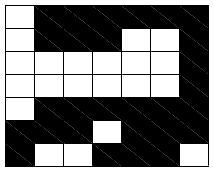
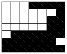
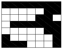
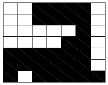
GOOD
GOOD
BAD
?
The choice of how to represent input is very important
Can we classify the unknown pattern?
Converting Pattern to Binary Vector
Binary Representation
x = 0111111011100100000010000
    001011111111101111001110
Label: “GOOD”
Key Insight
The same pattern can be represented as:
- Raw pixels
- Binary vectors (length d = 49)
- Feature vectors
- Learned representations
A hypothesis class can succeed or fail based on the choice of representation.
Linear vs Nonlinear Hypothesis Classes
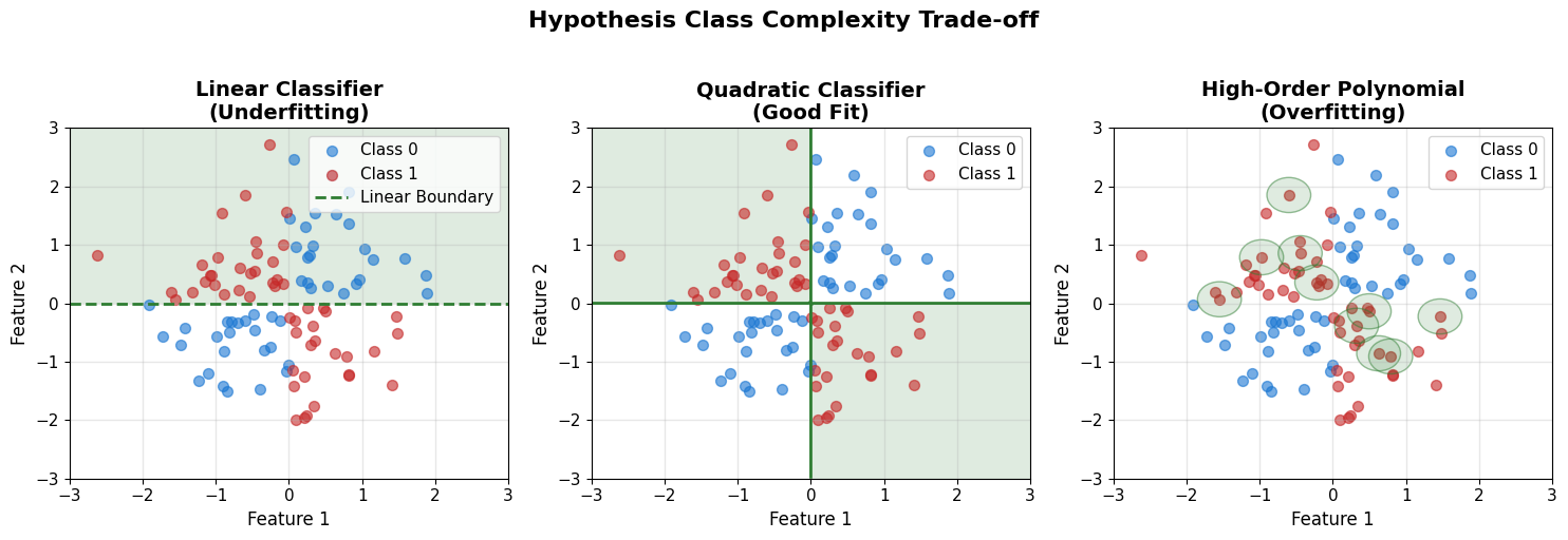
\[\mathcal{H}_{\text{linear}}: h(\mathbf{x}) = \text{sign}(\mathbf{w}^T\mathbf{x} + b)\]
\[\mathcal{H}_{\text{neural}}: h(\mathbf{x}) = h_2(\mathbf{W}_2 \cdot h_1(\mathbf{W}_1\mathbf{x} + \mathbf{b}_1) + \mathbf{b}_2)\]
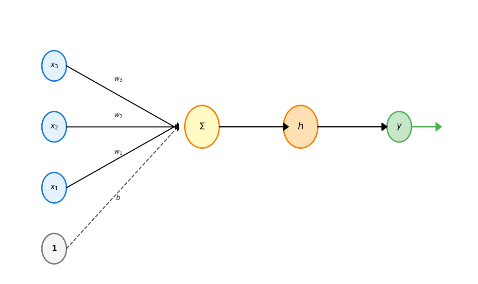
Perceptron: Linear Combination + Nonlinearity
Mathematical Model
\[y = h\left(\sum_{i=1}^n w_i x_i + b\right) = h(\mathbf{w}^T\mathbf{x} + b)\]
where \(h\) is an activation function:
- Step: \(h(z) = \begin{cases} 1 & z \geq 0 \\ 0 & z < 0 \end{cases}\)
- Sigmoid: \(h(z) = \frac{1}{1 + e^{-z}}\)
- ReLU: \(h(z) = \max(0, z)\)
Activation Functions Add Nonlinearity
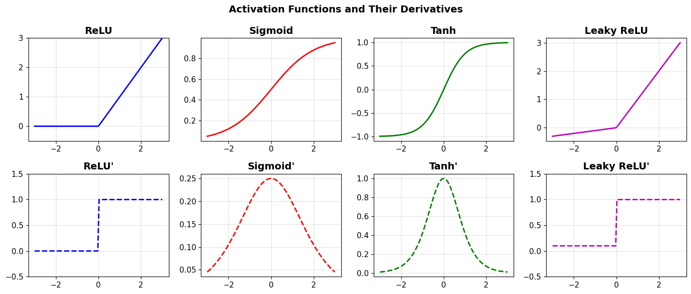
Why Nonlinearity Matters
Without activation functions, stacking layers is pointless: \(f(\mathbf{W}_2 \mathbf{W}_1 \mathbf{x}) = f(\mathbf{W} \mathbf{x})\) where \(\mathbf{W} = \mathbf{W}_2\mathbf{W}_1\)
Later topic: Gradient flow and vanishing gradients during backpropagation
Gradient Descent Visualization
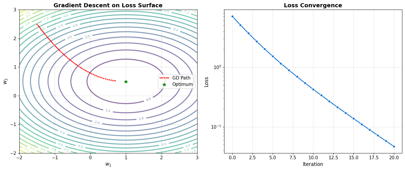
Iterative Optimization Principle
Gradient descent navigates the loss landscape by repeatedly moving in the direction of steepest descent. For convex problems, this guarantees convergence to the global minimum. For neural networks, we settle for local minima that generalize well.
The Bias-Variance Decomposition
Expected Prediction Error
\[\text{MSE} = \text{Bias}^2 + \text{Variance} + \sigma^2\]
Bias: Error from wrong model assumptions
- High bias: Model too simple (underfits)
- Low bias: Model captures true pattern
Variance: Error from sensitivity to training data
- High variance: Model memorizes noise (overfits)
- Low variance: Model finds generalizable pattern
Irreducible error (\(\sigma^2\)): Noise inherent in data
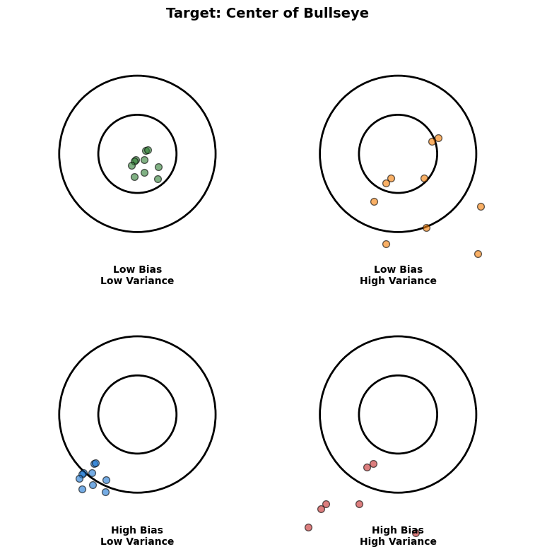
Tradeoff: Complex models reduce bias but increase variance
Bias-Variance in Practice: Polynomial Fitting
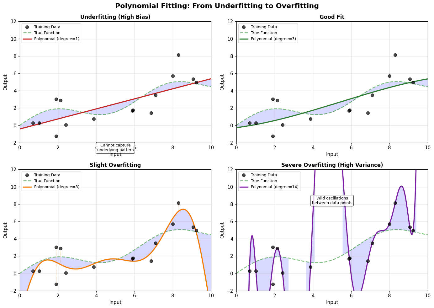
- Degree 1: Too simple, systematic error (high bias)
- Degree 3: Captures pattern without noise
- Degree 8: Starts fitting noise
- Degree 14: Wild oscillations (high variance)
Increasing complexity: bias decreases, variance increases
Representation Transforms Problem Difficulty
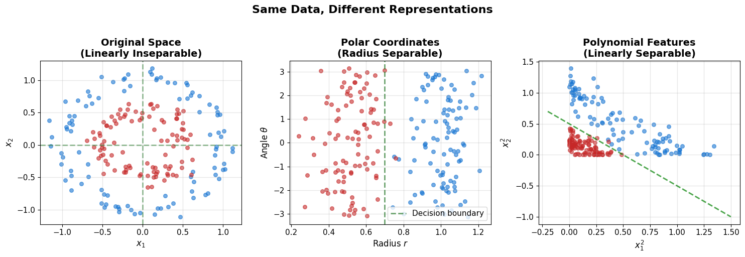
Representation Determines Learnability
Concentric circles: linearly inseparable in Cartesian coordinates, but trivially separable by radius in polar coordinates. Deep learning automates this search for effective representations.
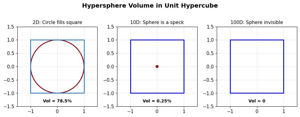
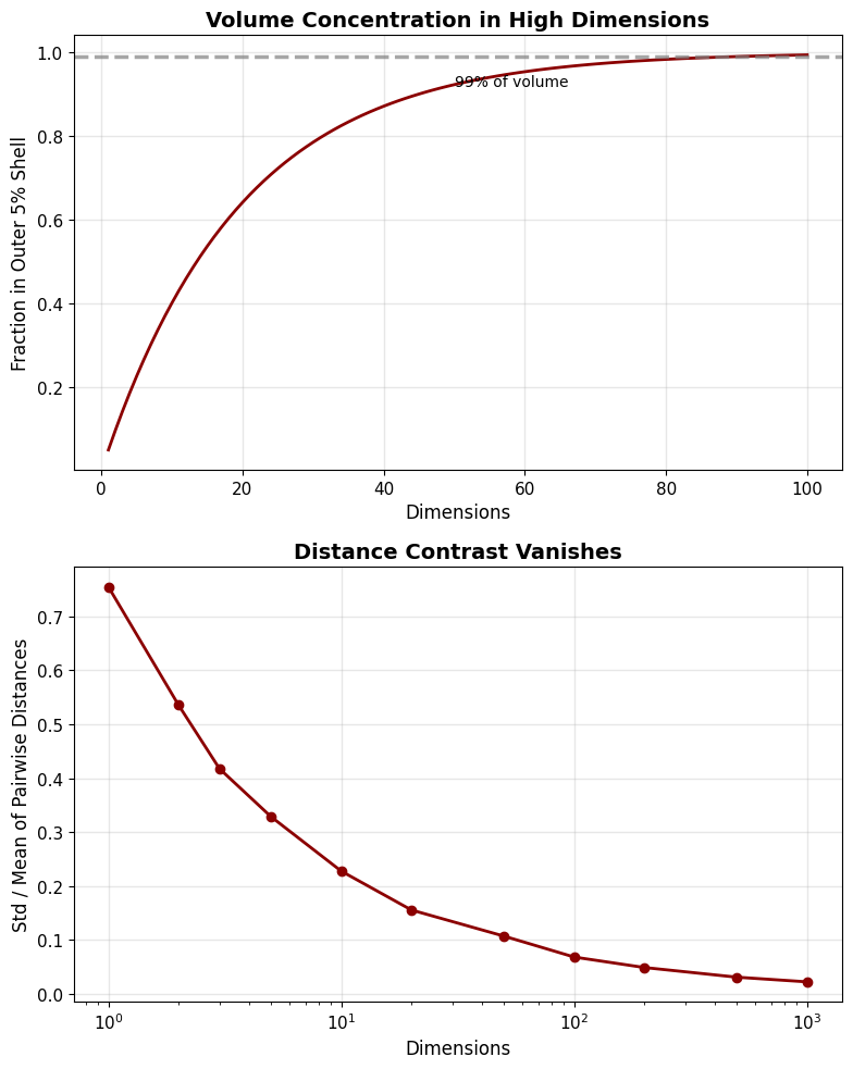
High Dimensions Break Geometric Intuition
The Curse of Dimensionality
As \(d \to \infty\):
- All points become equidistant
- Volume concentrates at surface
- Gaussian looks like uniform
- Nearest neighbors aren’t “near”
Code
import numpy as np

def volume_ratio(d, epsilon=0.95):
    """Fraction of hypercube volume in outer shell"""
    return 1 - epsilon**d

dimensions = [1, 2, 3, 10, 100, 1000]
for d in dimensions:
    ratio = volume_ratio(d)
    print(f"d={d:4}: {ratio:.6f} in outer shell")
d=   1: 0.050000 in outer shell
d=   2: 0.097500 in outer shell
d=   3: 0.142625 in outer shell
d=  10: 0.401263 in outer shell
d= 100: 0.994079 in outer shell
d=1000: 1.000000 in outer shell
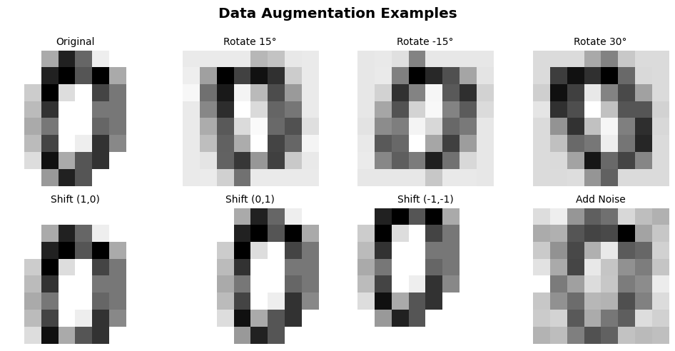
Data Augmentation: Synthetic Diversity from Limited Samples
Standard Augmentations
- Geometric: Rotation, flip, crop, scale
- Photometric: Brightness, contrast, color
- Noise: Gaussian, dropout, cutout
- Advanced: Mixup, CutMix, AutoAugment
Mathematical View
Training on augmented data:
\[\min_\theta \sum_{i=1}^N \sum_{j=1}^M \mathcal{L}(f_\theta(T_j(x_i)), y_i)\]
where \(T_j\) are augmentation transforms
Three Paradigms: Supervised, Unsupervised, Reinforcement
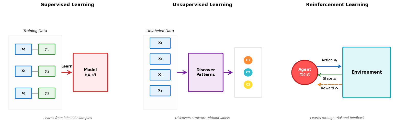
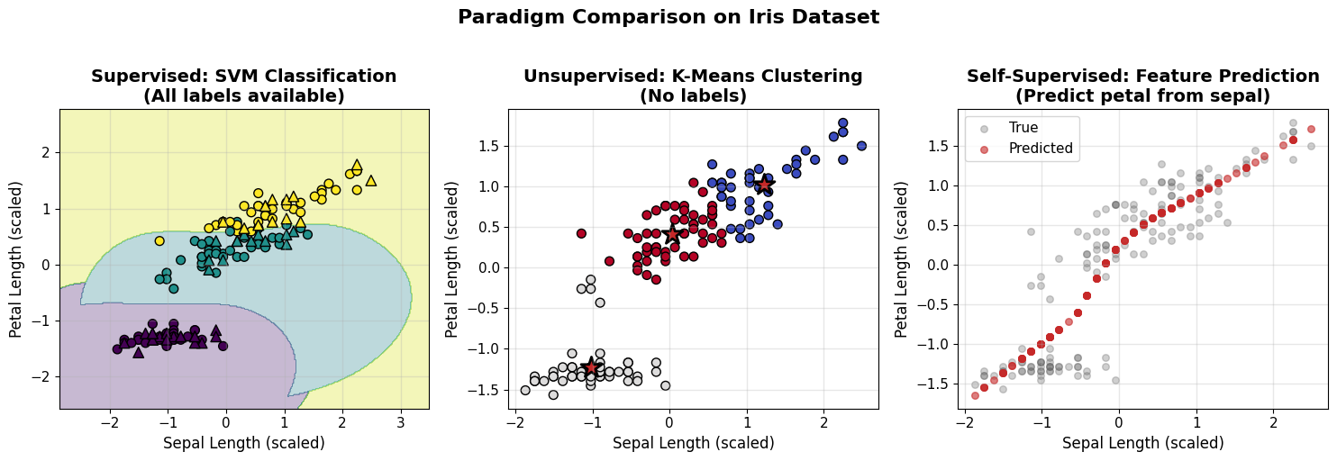
Modern methods combine paradigms: GPT-4 uses unsupervised pre-training on text, supervised fine-tuning on tasks, and reinforcement learning from human feedback (RLHF).
Supervised Learning Training and Inference
Training Phase
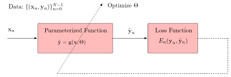
Inference Phase
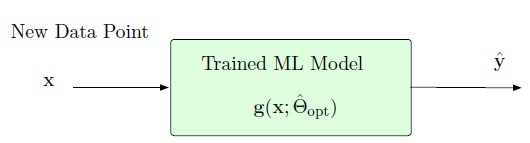
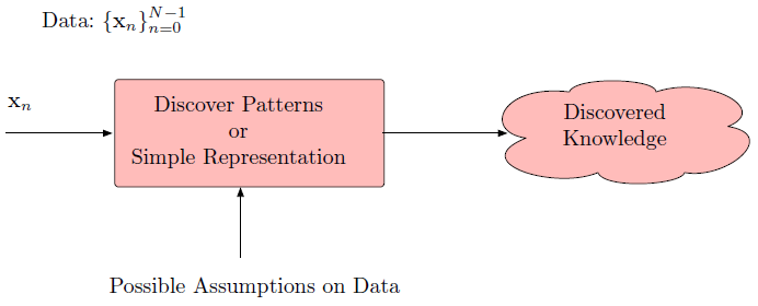
Unsupervised Learning: Structure from Unlabeled Data
No Labels, Just Data
Given: \(\mathcal{D} = \{\mathbf{x}_i\}_{i=1}^N\)
Find: Hidden patterns, structure, representations
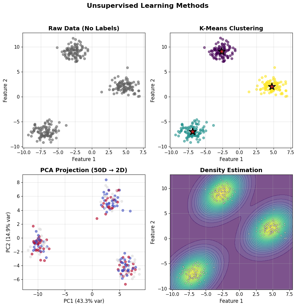
Key Methods
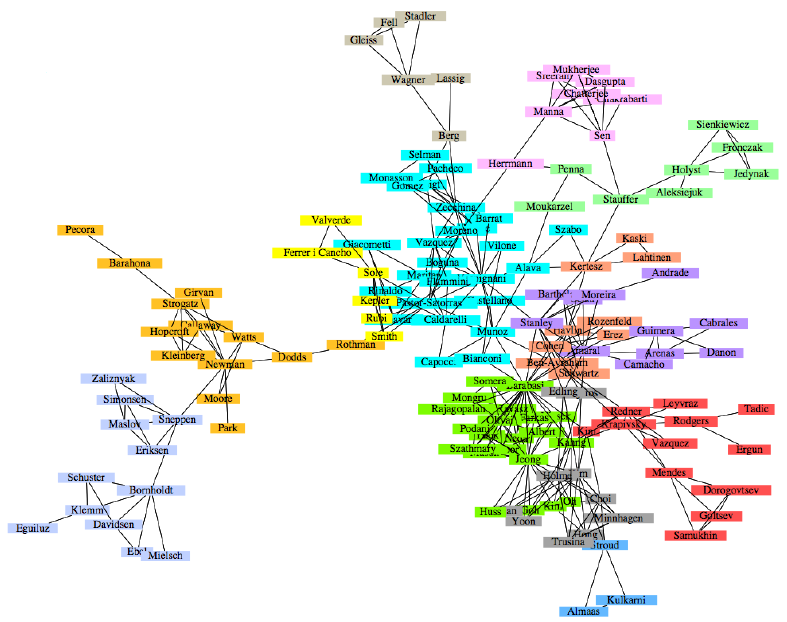
- Clustering: K-means, DBSCAN, hierarchical
- Dimensionality Reduction: PCA, t-SNE, UMAP
- Density Estimation: GMM, KDE
- Representation Learning: Autoencoders
Reinforcement Learning: Sequential Decision Making
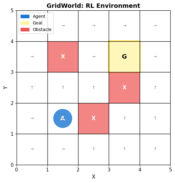
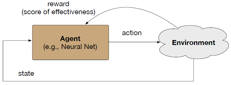
Sequential Decision Making
Components:
- State space: \(\mathcal{S}\)
- Action space: \(\mathcal{A}\)
- Reward function: \(R(s, a)\)
- Policy: \(\pi(a|s)\)
Objective: Maximize expected cumulative reward
\[J(\pi) = \mathbb{E}_{\pi}\left[\sum_{t=0}^{\infty} \gamma^t r_t\right]\]
Applications
- Game playing (Chess, Go, StarCraft)
- Robotics control
- Resource allocation
- Trading strategies
Same Problem, Different Paradigms
Label efficiency on CIFAR-10:
- Standard supervised training uses all 50,000 labels
- FixMatch (semi-supervised): 250 labels → 94.9% test accuracy; 40 labels → 88.6% [Sohn et al. 2020]
The other 49,750 unlabeled images carry most of the information — labels are the scarce resource.
Modern Methods Combine Paradigms
Semi-Supervised Learning
- Use small labeled + large unlabeled data
- Pseudo-labeling, consistency regularization
- Example: FixMatch, MixMatch
Multi-Task Learning
- Learn multiple related tasks simultaneously
- Shared representations
- Example: BERT for multiple NLP tasks
Meta-Learning
- Learn to learn
- Few-shot adaptation
- Example: MAML, Prototypical Networks
Transfer Learning Pipeline
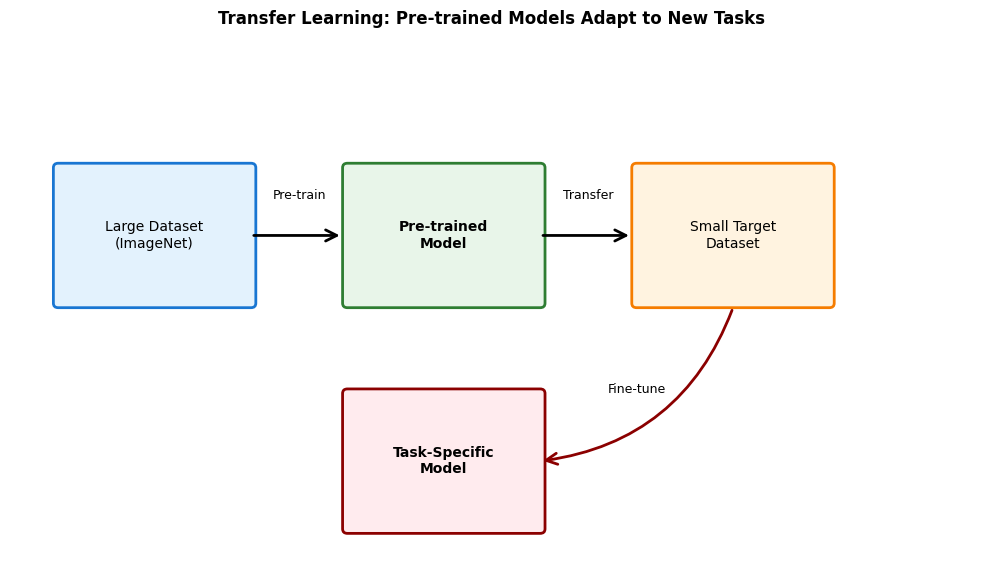
Hybrid Learning Approaches
Modern approaches often combine paradigms for better performance
Neural Networks Form a Rich Hypothesis Class
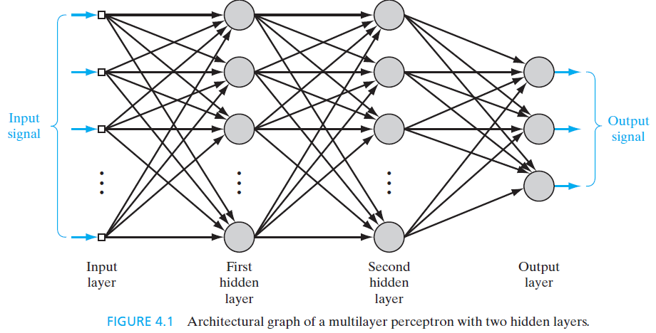
Multilayer Perceptron (MLP): Fully connected feedforward network
Architecture Components
- Input layer: Raw features \(\mathbf{x} \in \mathbb{R}^d\)
- Hidden layers: Learned representations
- Output layer: Task-specific predictions
- Connections: All-to-all between layers
Why “Rich” Hypothesis Class?
- Each neuron: Nonlinear transformation
- Composition: Exponential expressivity
- Universal approximation capability
Defn: Deep Neural Network
A neural network with more than one hidden layer. Depth enables hierarchical feature learning: early layers learn simple features, deeper layers learn complex abstractions.
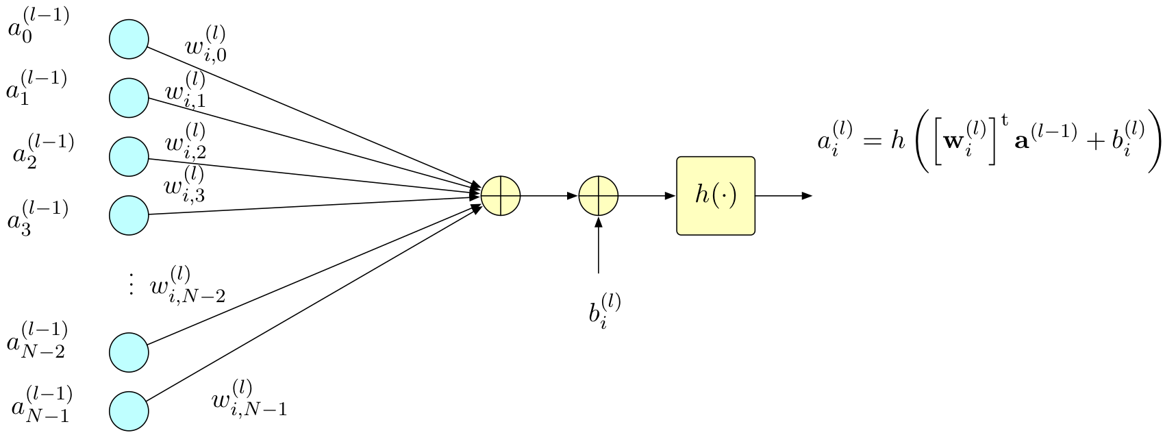
Single Neuron Computation
Forward Computation
At neuron \(i\) in layer \(l\):
\[a_i^{(l)} = h\left(\left[\mathbf{w}_i^{(l)}\right]^\top \mathbf{a}^{(l-1)} + b_i^{(l)}\right)\]
where:
- \(\mathbf{a}^{(l-1)}\): Previous layer activations
- \(\mathbf{w}_i^{(l)}\): Weight vector for neuron \(i\)
- \(b_i^{(l)}\): Bias term
- \(h(\cdot)\): Activation function
Matrix Form (Entire Layer)
\[\mathbf{a}^{(l)} = h\left(\mathbf{W}^{(l)} \mathbf{a}^{(l-1)} + \mathbf{b}^{(l)}\right)\]
- Parallelizes computation
- Enables GPU acceleration
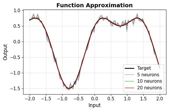
Universal Approximation: Existence Guarantee
Cybenko (1989), Hornik et al. (1989)
A feedforward network with:
- Single hidden layer
- Finite number of neurons
- Non-polynomial activation
can approximate any continuous function on compact subset of \(\mathbb{R}^n\) to arbitrary accuracy
Critical word: CAN
The theorem guarantees such networks exist. Finding them through training is different.
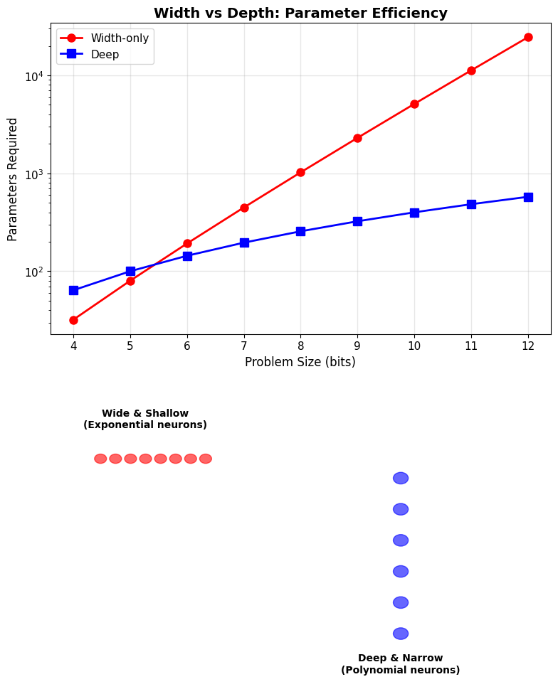
Width vs Depth: Why We Use Deep Networks
Width-only (single hidden layer)
Universal approximation guarantees this works, but:
- May require exponentially many neurons
- Example: parity function on n bits needs \(2^{n-1}\) hidden units
- Theorem says existence, not efficiency
Depth (multiple layers)
- More parameter-efficient representation
- Polynomial neurons vs exponential
- Hierarchical features emerge
- Same expressivity, fewer parameters
Why depth matters: Practical networks need efficient representations
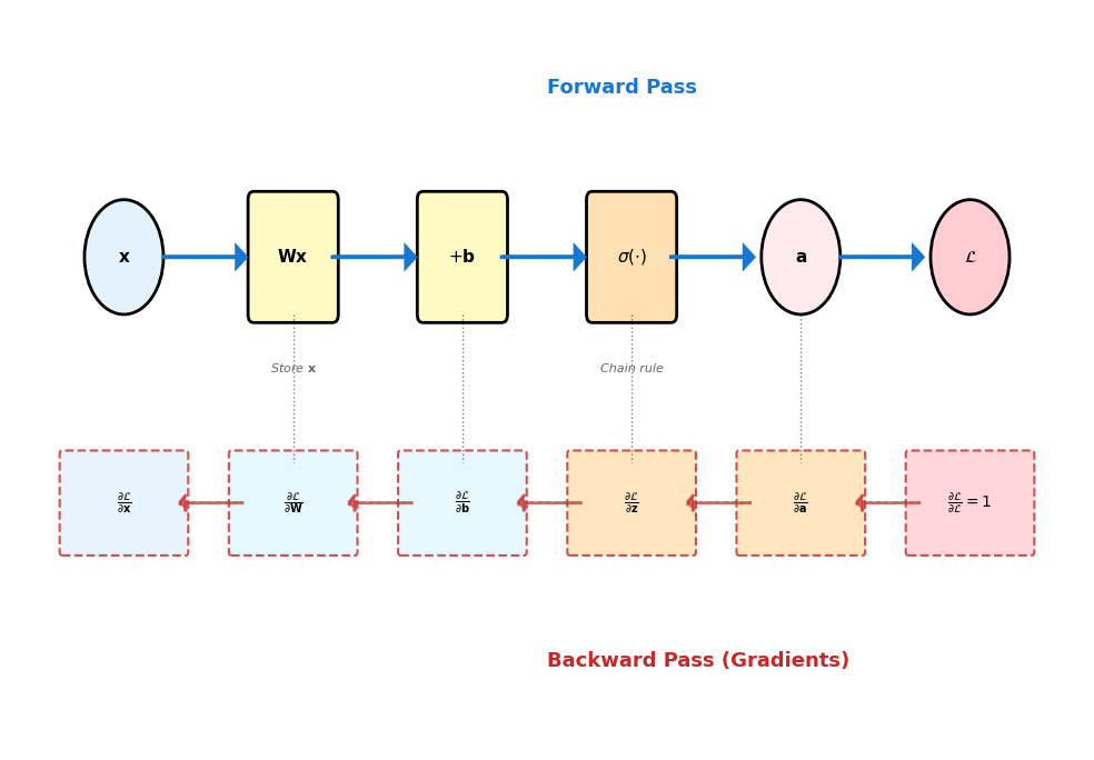
Forward and Backward Pass
Implementation
class Layer:
    def forward(self, x):
        # Store for backward pass
        self.x = x
        # Linear transformation
        self.z = np.dot(x, self.W) + self.b
        # Apply activation
        self.a = self.activation(self.z)
        return self.a

    def backward(self, grad_output):
        # Chain rule through activation
        grad_z = grad_output * \
                 self.activation_derivative(self.z)

        # Parameter gradients
        self.grad_W = np.dot(self.x.T, grad_z)
        self.grad_b = np.sum(grad_z, axis=0)

        # Input gradient for previous layer
        grad_input = np.dot(grad_z, self.W.T)
        return grad_input
Computational Graph
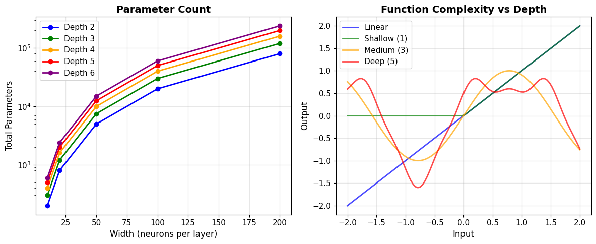
Network Capacity and Depth
Loss Surfaces in High Dimensions
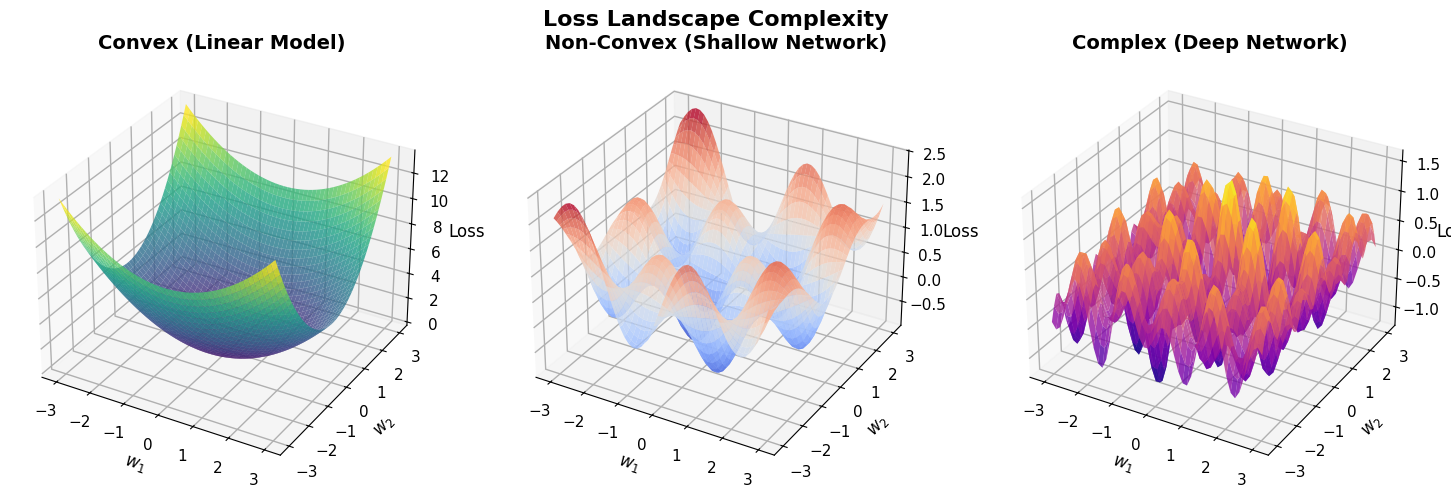
Mathematical Reality
In \(d\) dimensions with \(n\) parameters:
- Critical points: \(\mathcal{O}(e^n)\)
- Most are saddle points, not local minima
- Minima often connected by low-loss paths
Empirical Observations
- Loss landscapes are surprisingly well-behaved
- Wide networks have smoother landscapes
- Overparameterization helps optimization
- Mode connectivity phenomenon
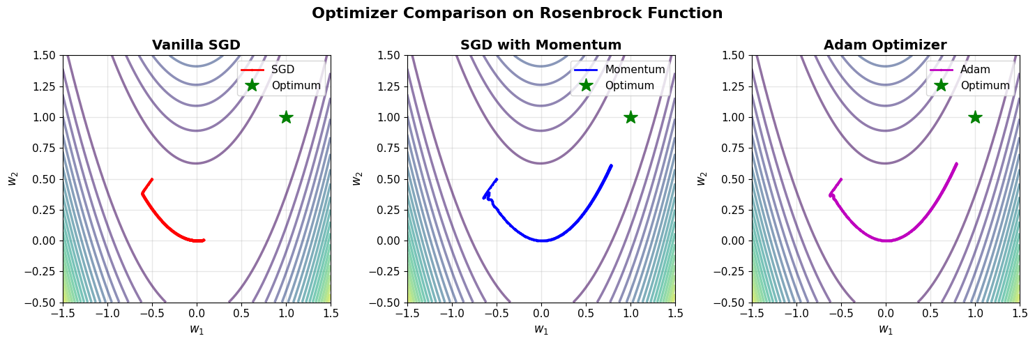
Stochastic Gradient Descent and Variants
Code
def sgd(w, grad, lr=0.01):
    return w - lr * grad

def sgd_momentum(w, grad, velocity, lr=0.01, beta=0.9):
    velocity = beta * velocity + lr * grad
    return w - velocity, velocity

def adam(w, grad, m, v, t, lr=0.001, beta1=0.9, beta2=0.999, eps=1e-8):
    m = beta1 * m + (1 - beta1) * grad
    v = beta2 * v + (1 - beta2) * grad**2
    m_hat = m / (1 - beta1**t)
    v_hat = v / (1 - beta2**t)
    return w - lr * m_hat / (np.sqrt(v_hat) + eps), m, v
Lottery Ticket Hypothesis: Sparse Subnetworks at Initialization
Frankle & Carbin (2019)
“Dense networks contain sparse subnetworks that can train to comparable accuracy from the same initialization”
Implications
- Networks are vastly overparameterized
- Winning tickets exist at initialization
- Pruning can maintain performance
- Structure matters more than we thought
Practical Impact
\[\text{Parameters: } 100M \to 10M\]
\[\text{Performance: } 95\% \to 94.5\%\]
Why this matters:
Storage:
- 100M: ~400MB (too large for mobile)
- 10M: ~40MB (fits on phone)
Speed:
- 100M: ~100ms per image
- 10M: ~10ms per image (real-time)
Training:
- 100M: 5 days on single GPU
- 10M: 12 hours (faster experiments)
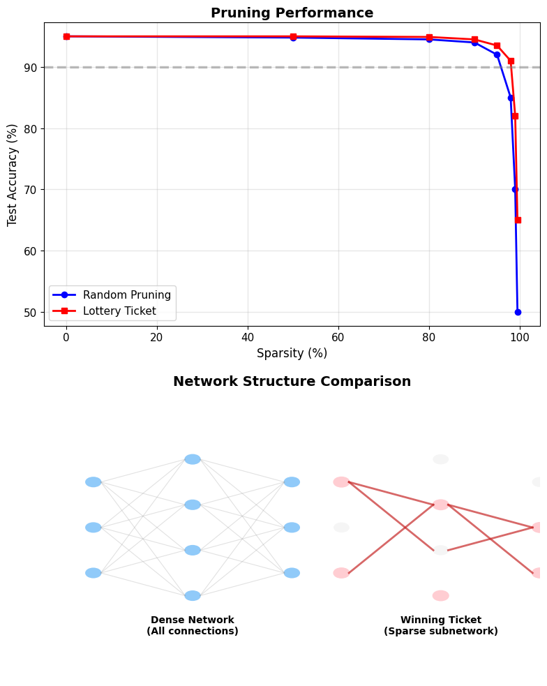
Detailed treatment: Network pruning and efficient architectures
More Parameters Can Mean Better Generalization
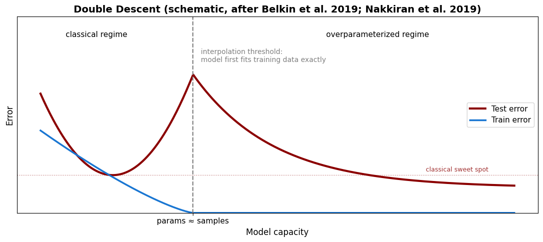
Past the point of an exact fit, test error descends again — networks with many times more parameters than training samples routinely generalize best. The classical bias–variance picture describes the left half only.
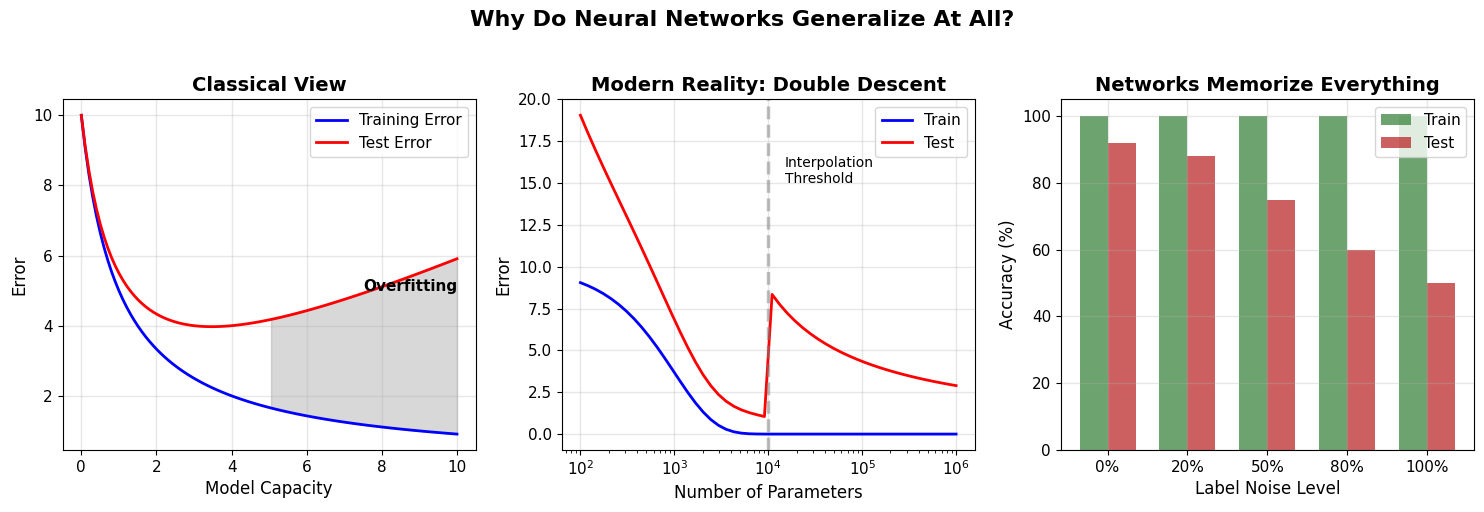
Neural Networks Memorize Random Labels Yet Generalize on Real Data
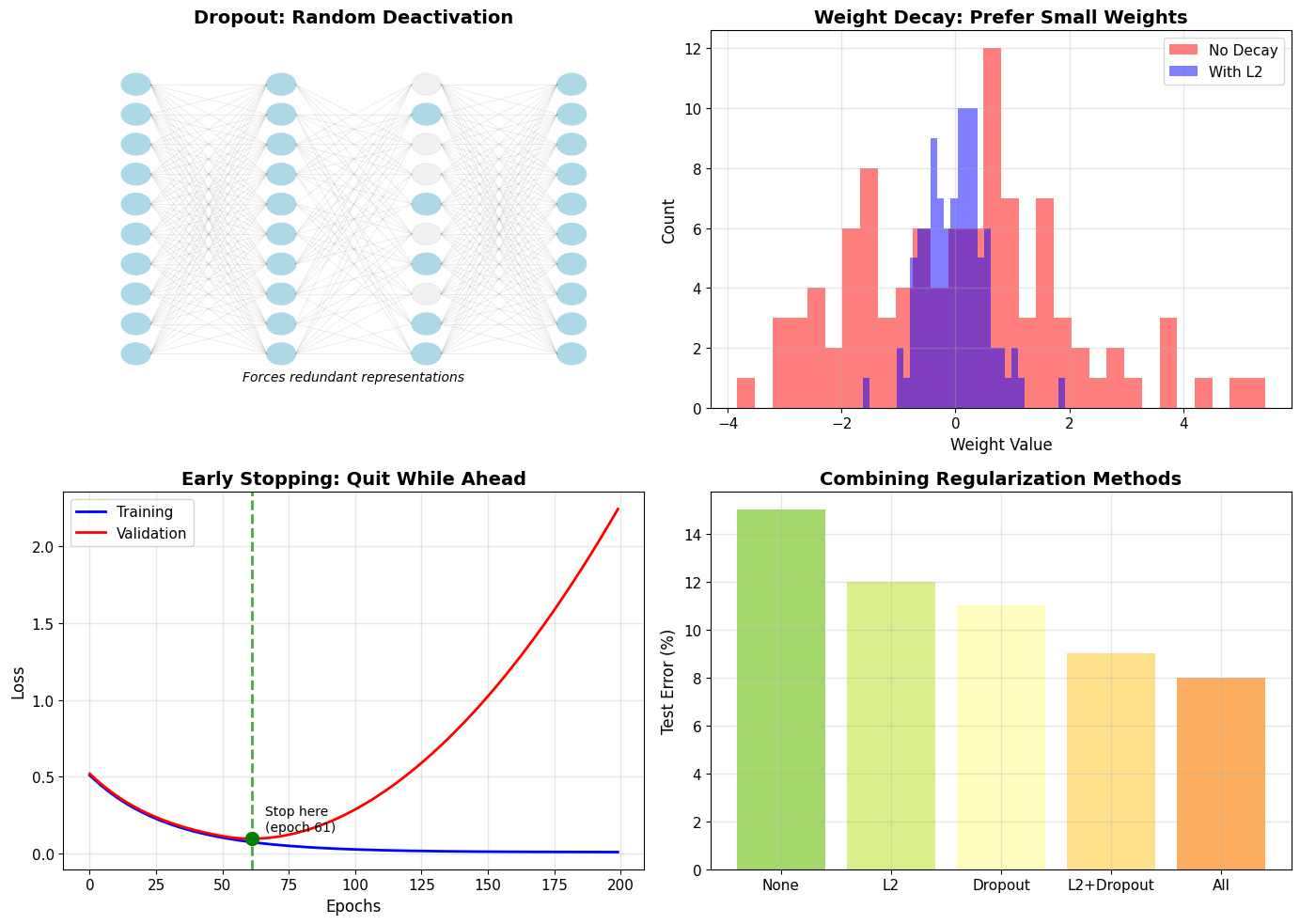
Regularization Techniques: Dropout and Weight Decay
def dropout(x, p=0.5, training=True):
    if not training:
        return x
    mask = np.random.binomial(1, 1-p, size=x.shape) / (1-p)
    return x * mask

def weight_decay(loss, weights, lambda_reg=0.01):
    l2_penalty = sum(np.sum(w**2) for w in weights)
    return loss + lambda_reg * l2_penalty
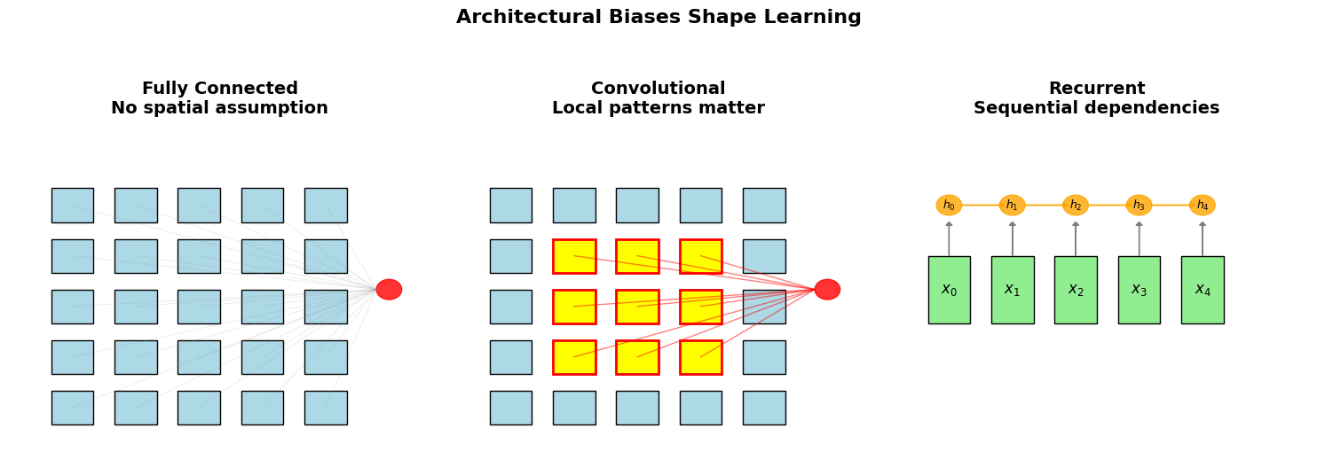
Architecture Embeds Domain Knowledge
Train/Validation/Test: Separation Is Sacrosanct
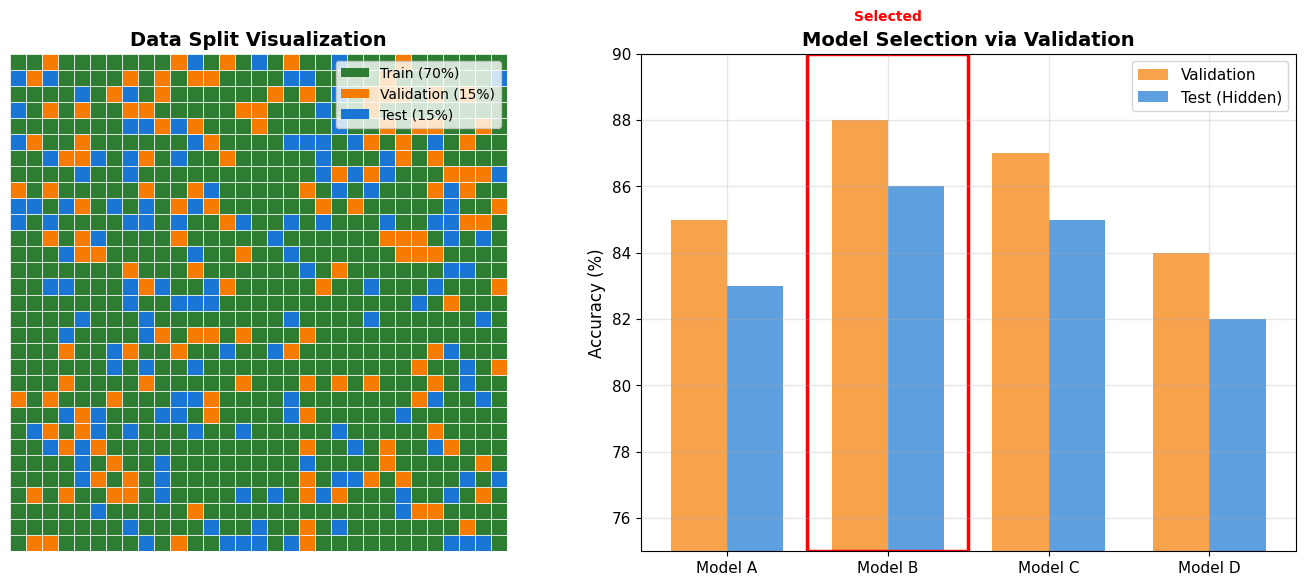
WARNING: Data Contamination
Never touch test data until final evaluation - validation data guides all decisions
Zillow Home Pricing: When the World Changes
The system (2018–2021):
- Zillow Offers: buy homes at model-estimated prices, renovate, resell
- Zestimate-driven offers, scaled to thousands of homes per quarter
What went wrong (2021):
- Q3 purchases were priced above the company’s own later estimates of resale value
- Average gross loss per home sold in Q3: $80,771 across 3,032 homes
- Inventory write-down: $304M, with further losses expected on remaining inventory
Outcome: Zillow Offers wound down 02 November 2021; roughly 25% workforce reduction.
“The unpredictability in forecasting home prices far exceeds what we anticipated.” — Rich Barton, CEO
Zillow Group Q3 2021 results and shareholder letter, 02 November 2021.
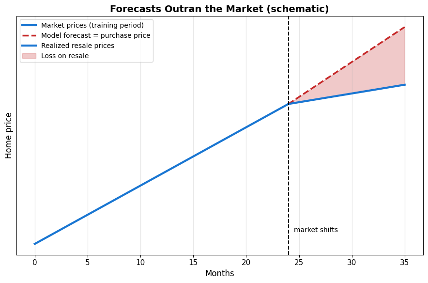
The problem:
All your validation tools assume the future looks like the past. When the world changes, models trained on historical data fail.
Train/val/test all from 2018-2020: Model learns pre-COVID patterns
Deploy in 2021: COVID changed everything
Result: Model is wrong, but doesn't know it's wrong
This is not a rare edge case - markets shift, user behavior changes, new products emerge. Distribution shift is common.
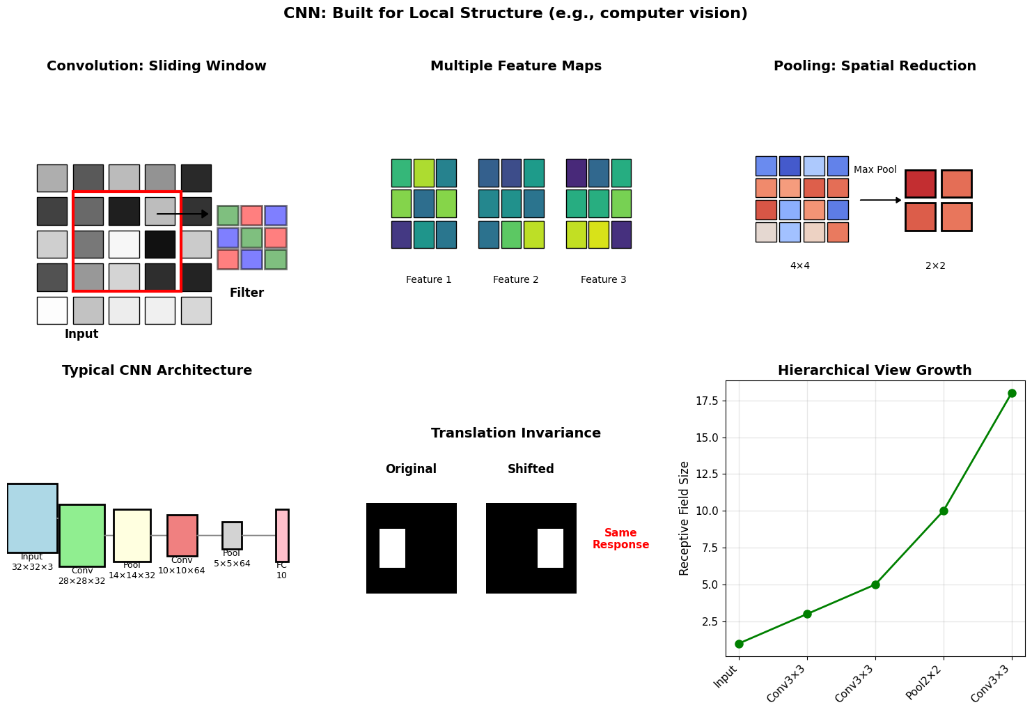
Convolutional Networks: Exploiting Spatial Structure
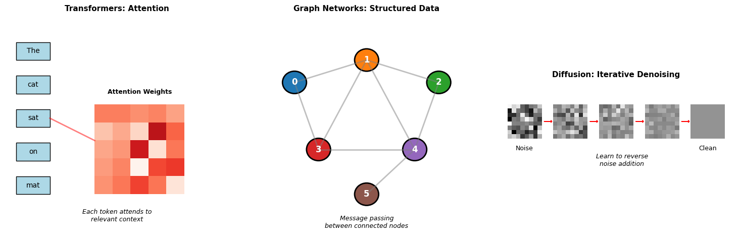
Preview: Transformers, Graph Networks, and Diffusion Models
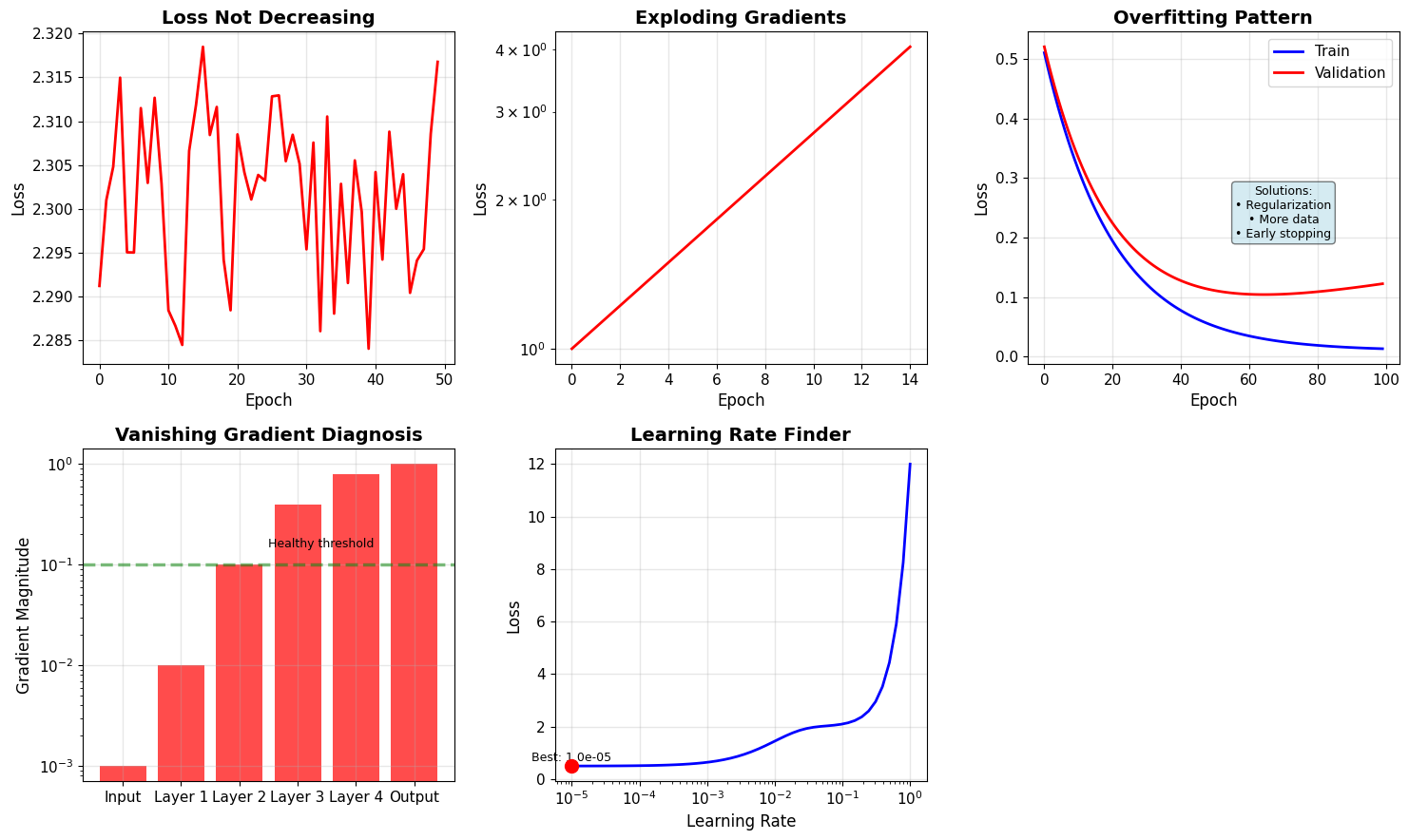
Debugging Deep Learning
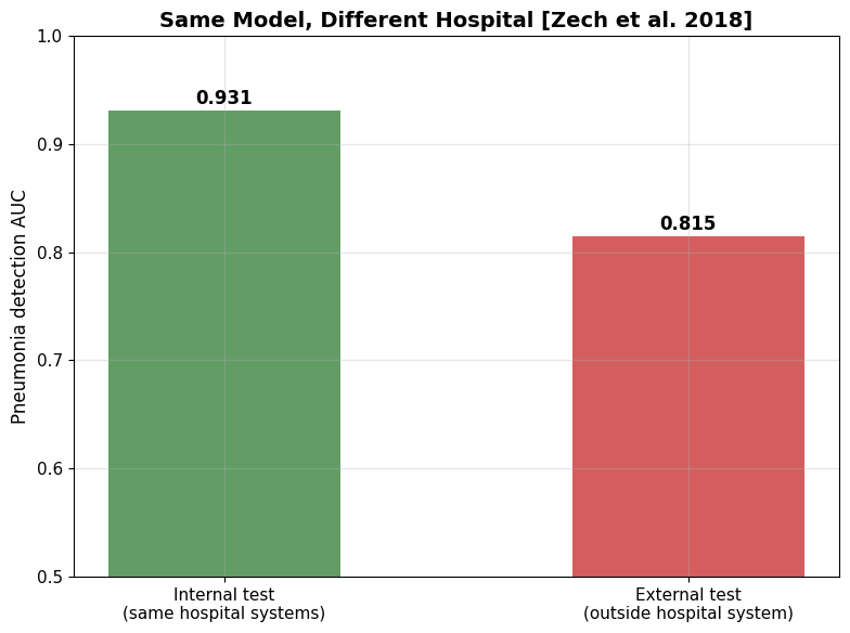
Medical Imaging: High Accuracy Hides Dataset Problems
The study [Zech et al., PLOS Medicine 2018]:
- Pneumonia detectors trained on 158,323 chest X-rays from three US systems (NIH, Mount Sinai, Indiana)
- Internal test AUC: 0.931
- Same model tested at an outside system: 0.815
- Significantly worse externally in 3 of 5 site comparisons
What the models keyed on:
- CNNs identified the acquiring hospital system from the image with near-perfect accuracy
- Departmental artifacts: portable-machine markers, laterality tokens, image processing style
- Site-specific pneumonia prevalence leaked into the score
Shortcut learning: Standard debugging looked fine:
- Training loss decreasing smoothly
- No overfitting (train/val gap small)
- High validation accuracy
- Good precision/recall on test set
Problem only appeared on different hospital equipment. Models exploit spurious correlations (disease + specific machine) as shortcuts instead of learning actual medical patterns.
Computational Realities
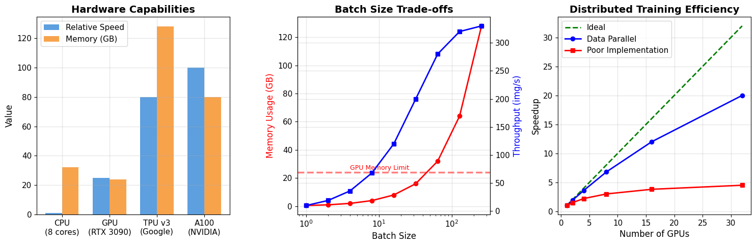
What this means for this course:
CPU (your laptop):
- Sufficient for: Most course assignments including smaller CNNs
- Time scale: Minutes per epoch on MNIST, tens of minutes on CIFAR-10
- Cost: Free
GPU (Colab/Kaggle free tier):
- Useful for: Faster iteration, larger architectures, final project
- Time scale: Seconds per epoch
- Cost: Free (with session limits)
Multi-GPU (cloud):
- Rarely needed: Only for very large-scale experiments
- Cost: $1-3 per hour
Course approach: CPU is viable for most work. GPU accelerates but isn’t required.
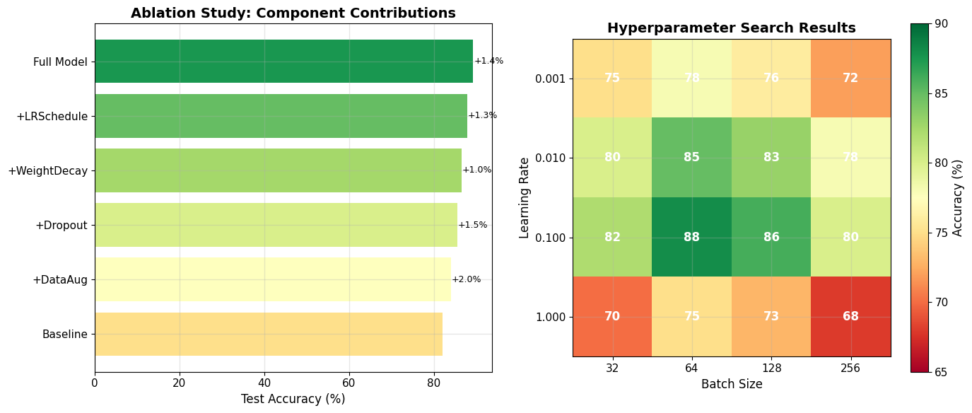
Systematic Experimentation
Experiment tracking example
# Tracking experiments
experiment_config = {
    'model': 'resnet18',
    'dataset': 'cifar10',
    'batch_size': 128,
    'lr': 0.1,
    'epochs': 100,
    'seed': 42,
    'timestamp': '2025-01-15-14:30'
}

# Always set seeds for reproducibility
def set_all_seeds(seed=42):
    np.random.seed(seed)
    # torch.manual_seed(seed)
    # torch.cuda.manual_seed_all(seed)
    # random.seed(seed)

# Log everything
def log_metrics(epoch, train_loss, val_loss, val_acc):
    metrics = {
        'epoch': epoch,
        'train_loss': train_loss,
        'val_loss': val_loss,
        'val_acc': val_acc,
        'lr': get_current_lr(),
        'timestamp': time.time()
    }
    # Write to file, tensorboard, wandb, etc.
    return metrics
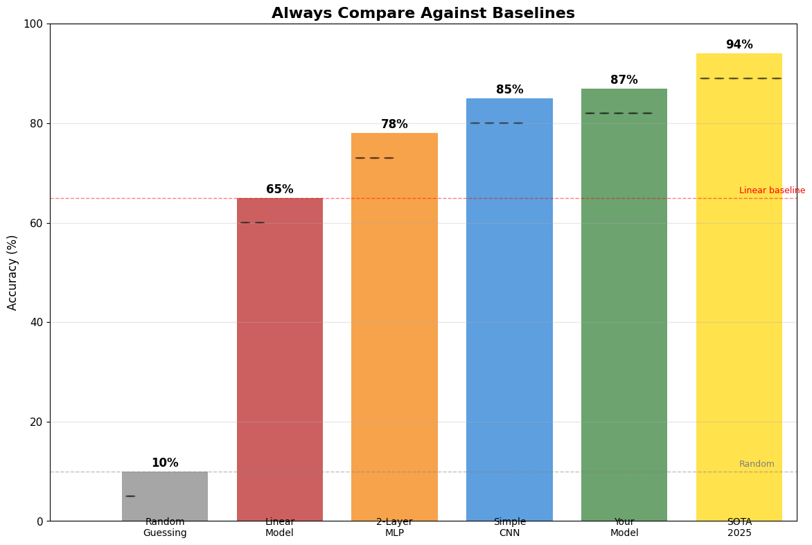
Always Establish Baselines Before Claiming Improvement
Course Architecture: Statistical to Neural
Scaling Laws and Emergent Capabilities
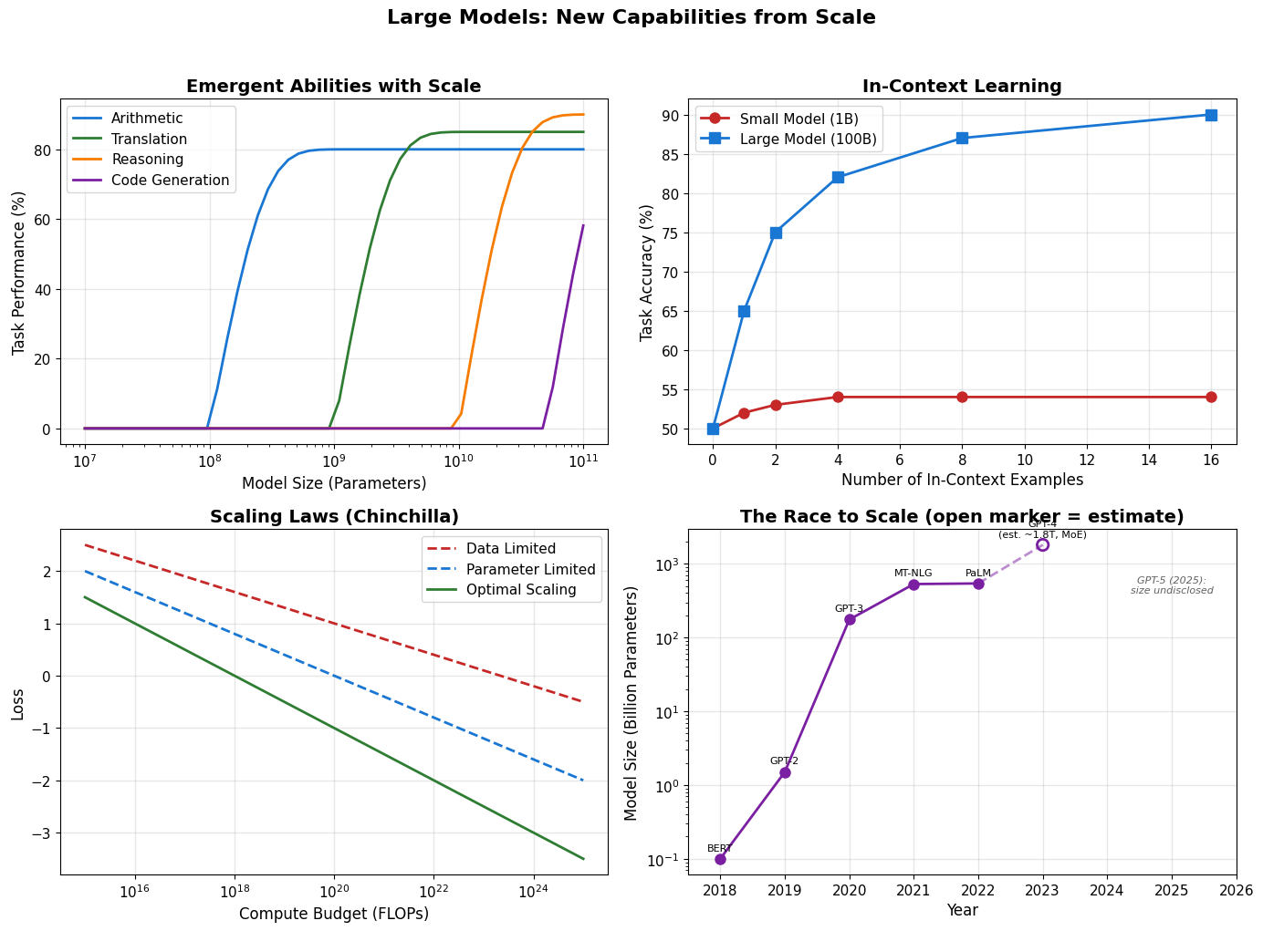
What these scales cost:
GPT-2 (1.5B params, 2019):
- Training: ~$50K compute, weeks on multi-GPU
- Inference: Runs on laptop CPU
GPT-3 (175B params, 2020):
- Training: ~$5M compute, months on cluster
- Inference: Requires GPU server
PaLM (540B params, 2022):
- Training: ~$10M+ compute, specialized infrastructure
- Inference: Multi-GPU required
GPT-4 (2023, size undisclosed — est. ~1.8T mixture-of-experts):
- Training: “more than $100M” per OpenAI’s CEO
- Inference: datacenter-scale serving
Scale is not just about bigger numbers - it’s about fundamentally different resource requirements. (GPT-5, 2025: no size or cost disclosed.)
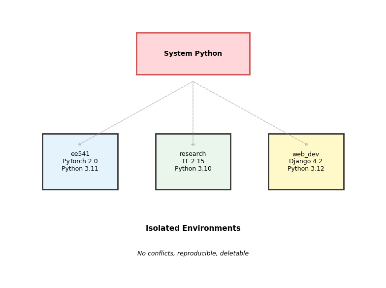
Environment Management: Why It Matters
Dependency Conflicts
# System Python - Don't do this
python install torch
# Error: requires numpy>=1.19
pip install numpy==1.20
# Breaks: opencv requires numpy==1.18
Conflicts are inevitable. Each project needs:
- Specific Python version
- Specific package versions
- Isolated from system Python
Virtual Environments
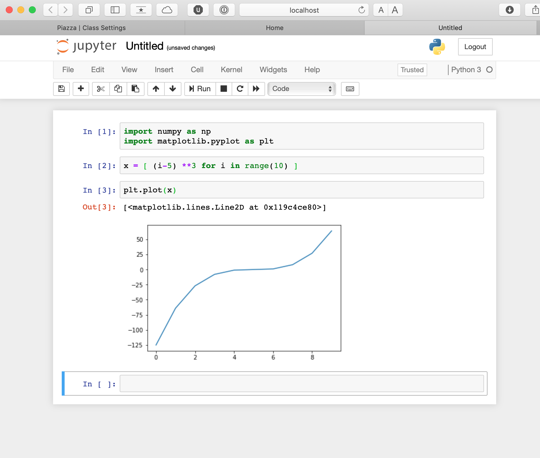
Jupyter Notebooks: Interactive Development
Starting Jupyter
# From terminal with environment active
(ee541) $ jupyter notebook

# Opens browser at localhost:8888
# Navigate to your work directory
Notebook Structure
- Cells: Code or Markdown
- Kernel: Python process executing code
- State: Variables persist between cells
Key Shortcuts
Shift+Enter: Run cell, move to nextCtrl+Enter: Run cell, stayEsc: Command modeEnter: Edit modeA/B: Insert cell above/below
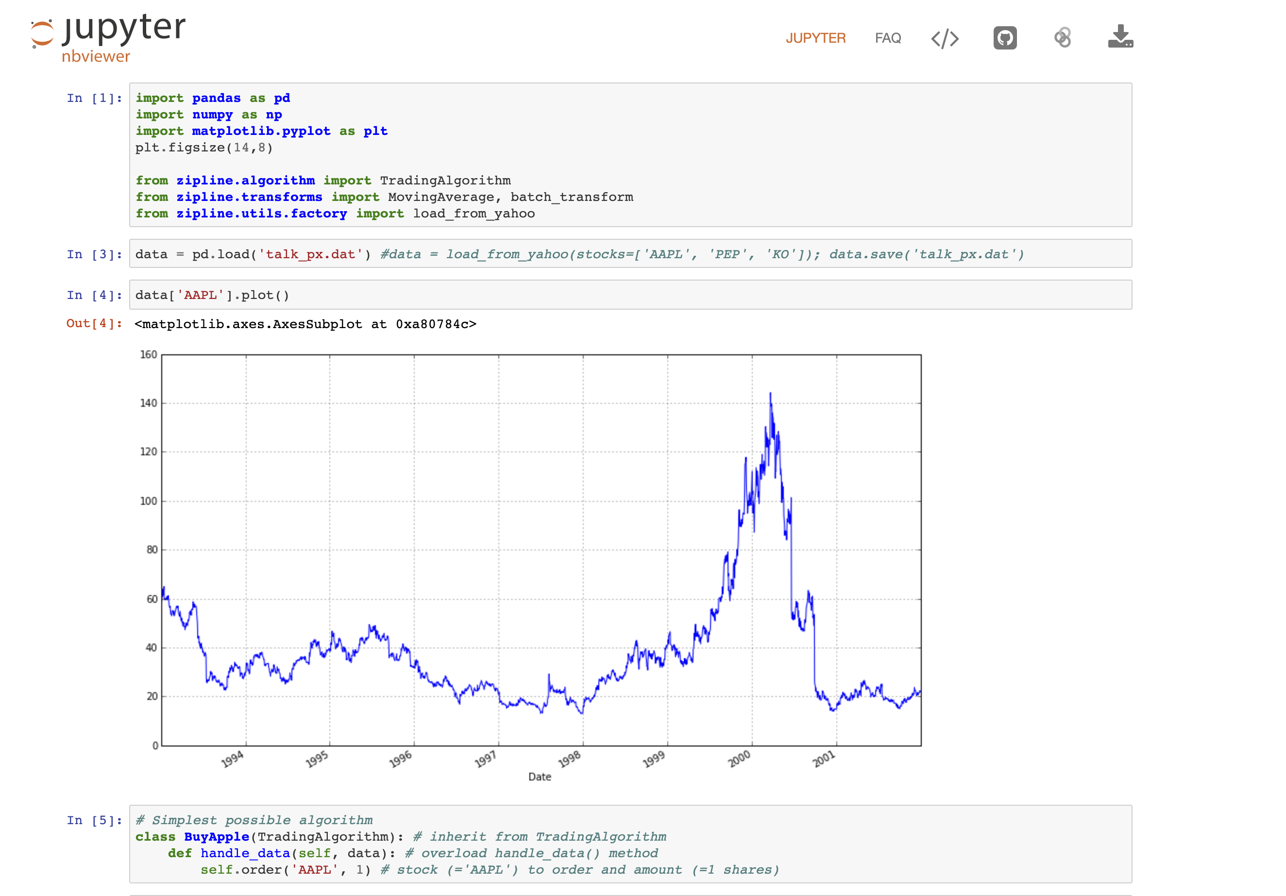
Real-World Example: Trading Algorithm
Project Management
Version Control
git init
git add .
git commit -m "Initial commit"

# But exclude:
# .gitignore contents:
*.pyc
__pycache__/
.ipynb_checkpoints/
data/
*.pt
*.pth
Reproducibility
# Save environment
conda env export > environment.yml

# Recreate elsewhere
conda env create -f environment.yml

# Save pip requirements
pip freeze > requirements.txt
Fashion-MNIST: 87% Accuracy in Four Epochs
What We’re Building
Task: Classify clothing items into 10 categories
Architecture: Simple 2-layer network
- Input: 28×28 grayscale images (784 pixels)
- Hidden: 128 neurons with ReLU
- Output: 10 classes (softmax)
Training: 4 epochs, Adam optimizer
Files:
1-fashion-mnist.ipynb: Dataset exploration2-minimal-pytorch.ipynb: Core training loop3-feature-visualization.ipynb: TensorBoard monitoring

T-shirt

Trouser

Pullover

Dress

Coat

Sandal

Shirt

Sneaker

Bag

Boot
Training Dynamics
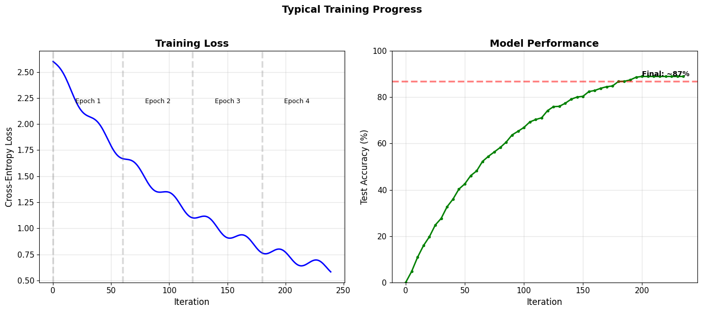
Observations:
- Rapid initial learning (first epoch)
- Diminishing returns with more training
- Test accuracy plateaus around 87% for this simple model
TensorBoard Visualization
Launch TensorBoard
# From terminal
tensorboard --logdir runs
# Navigate to http://localhost:6006
Available Visualizations
- Scalars: Loss, accuracy over time
- Images: Sample predictions
- Graph: Network architecture
- Embeddings: Feature space (PCA/t-SNE)
- Histograms: Weight distributions
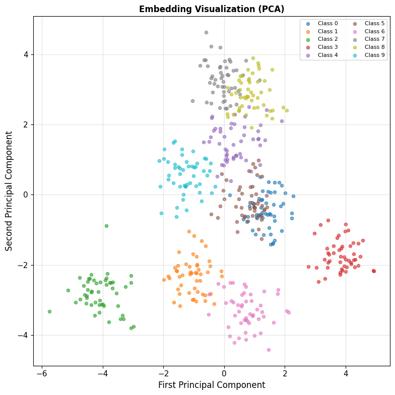
Embedding Insight: Classes form distinct clusters in feature space
Model Architecture Inspection
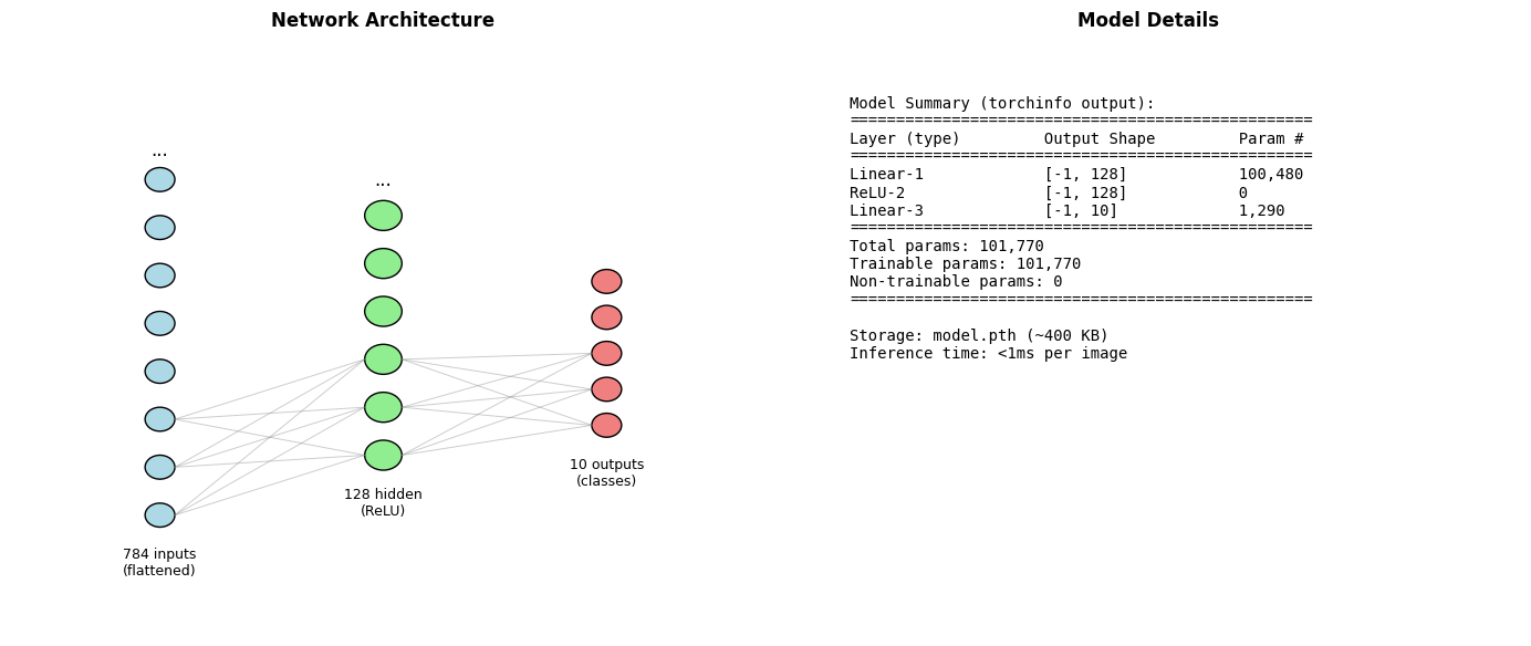
87% Accuracy Achieved with Simple Architecture
Implementation Results
- Model: 2-layer MLP with 128 hidden units
- Performance: 87% test accuracy after 4 epochs
- Training time: ~2 minutes on CPU
- Bottom line: Simple architectures work well for Fashion-MNIST
Not Addressed (Future Topics)
- Overfitting analysis: No train/val split comparison
- Hyperparameter tuning: Fixed learning rate, no grid search
- Architecture search: Only tried one configuration
- Regularization: No dropout, weight decay, or data augmentation
- Optimizer exploration: Only tried Adam, not SGD variants or AdamW
Main Files
1-fashion-mnist.ipynb      # Dataset exploration
2-minimal-pytorch.ipynb    # Core training
3-feature-visualization.ipynb  # TensorBoard
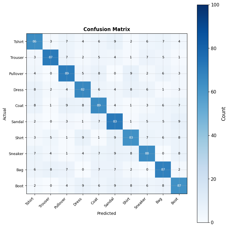
Common Confusions: Shirt ↔ T-shirt, Pullover ↔ Coat
Python and NumPy for Neural Networks
Next week: Array operations and automatic differentiation